Figures and data in The ‘German Job Miracle’ and Its Impact on Income Inequality: A Decomposition Study

Abstract

In the last 15 years before the COVID-19 crisis, Germany has experienced a strong and continuous increase in employment - the ‘German job miracle’. During this period, income inequality, which had previously increased sharply, remained relatively stable. This paper analyzes the impact of employment changes on disposable income inequality between 2004 and 2015 and gives an answer to the question why inequality remained constant despite the dramatic increase in employment. It is the first study to examine the effect of changing labor supply patterns due to changes in policies, wages and preferences, as well as the role that labor market constraints have played for inequality of disposable income. It finds that inequality would have increased further due to a transforming population structure, but increasing employment and policy changes almost completely offset this development. The results show that employment growth due to the reduction of labor market constraints has been more important in slowing down the increase in inequality than changes in labor supply.

This article contains 6 figures and 18 tables.

Figures

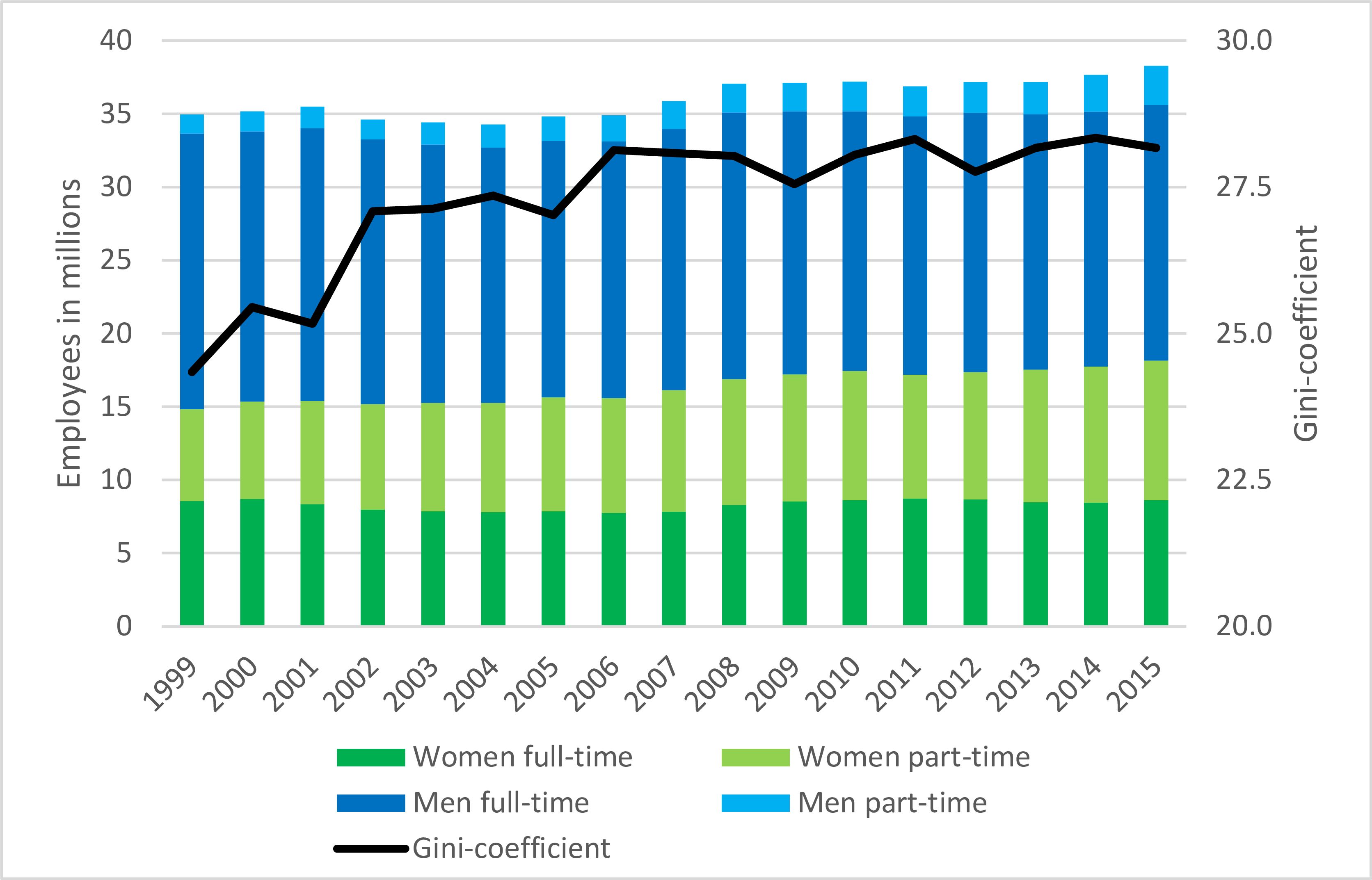
**Figure 1.** Trends in inequality and employment in Germany. Note: Inequality of equivalized disposable household income. Employment numbers includes the full population and self-employment.Source: SOEP v32.1; author’s own presentation.

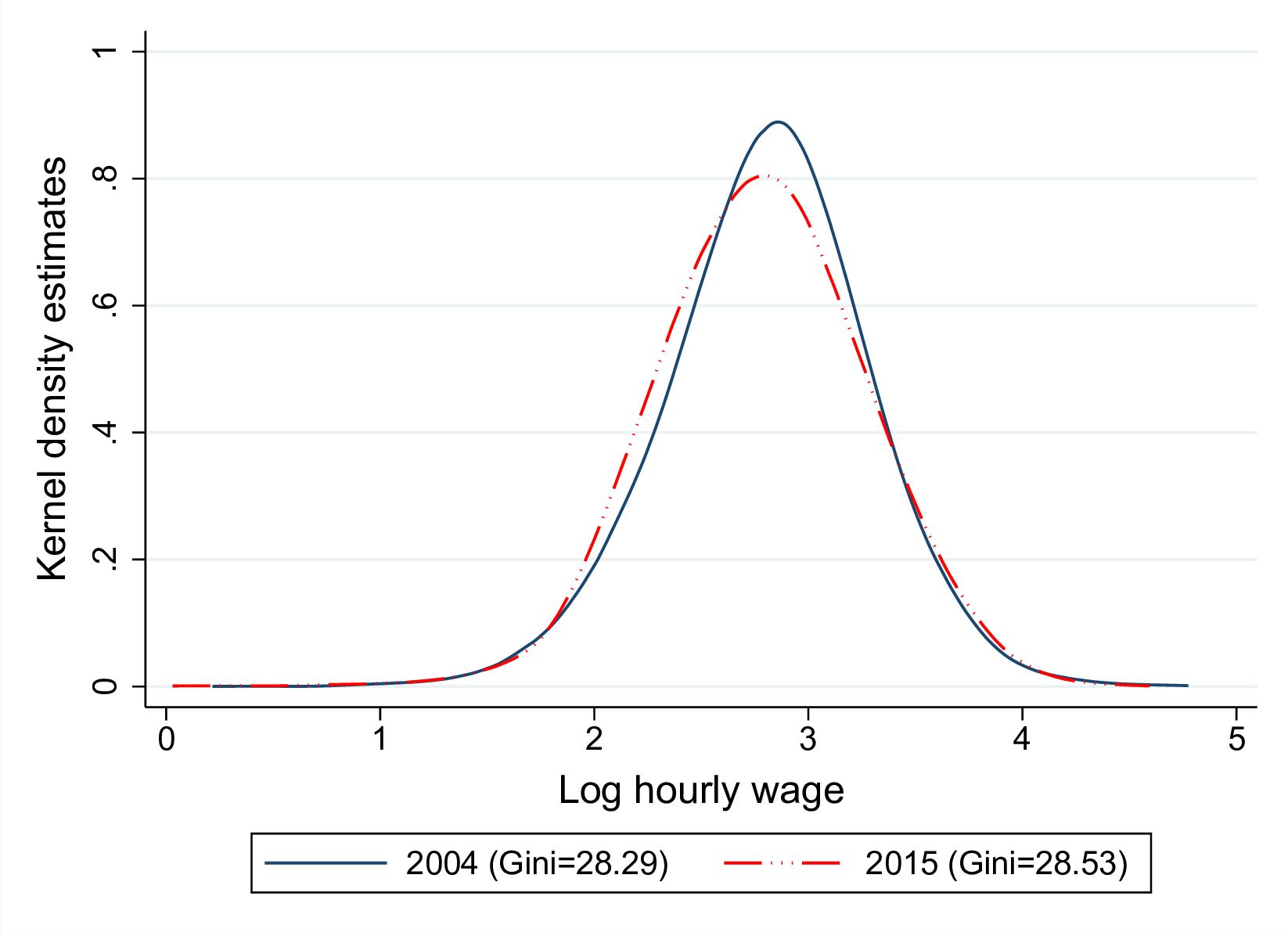
**Figure 2.** Kernel density estimate of log hourly wages for 2004 and 2015. Source: IAB-MSM; author’s own presentation.

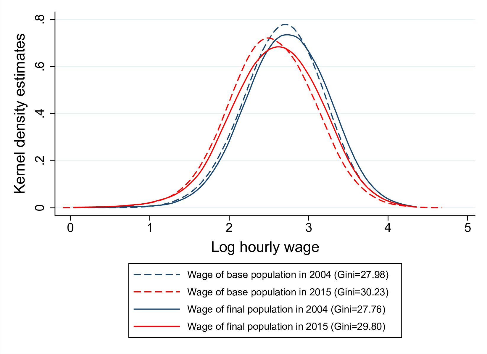
**Figure 3.** Simulated kernel density estimate of log hourly wages. Source: IAB-MSM; author’s own presentation.

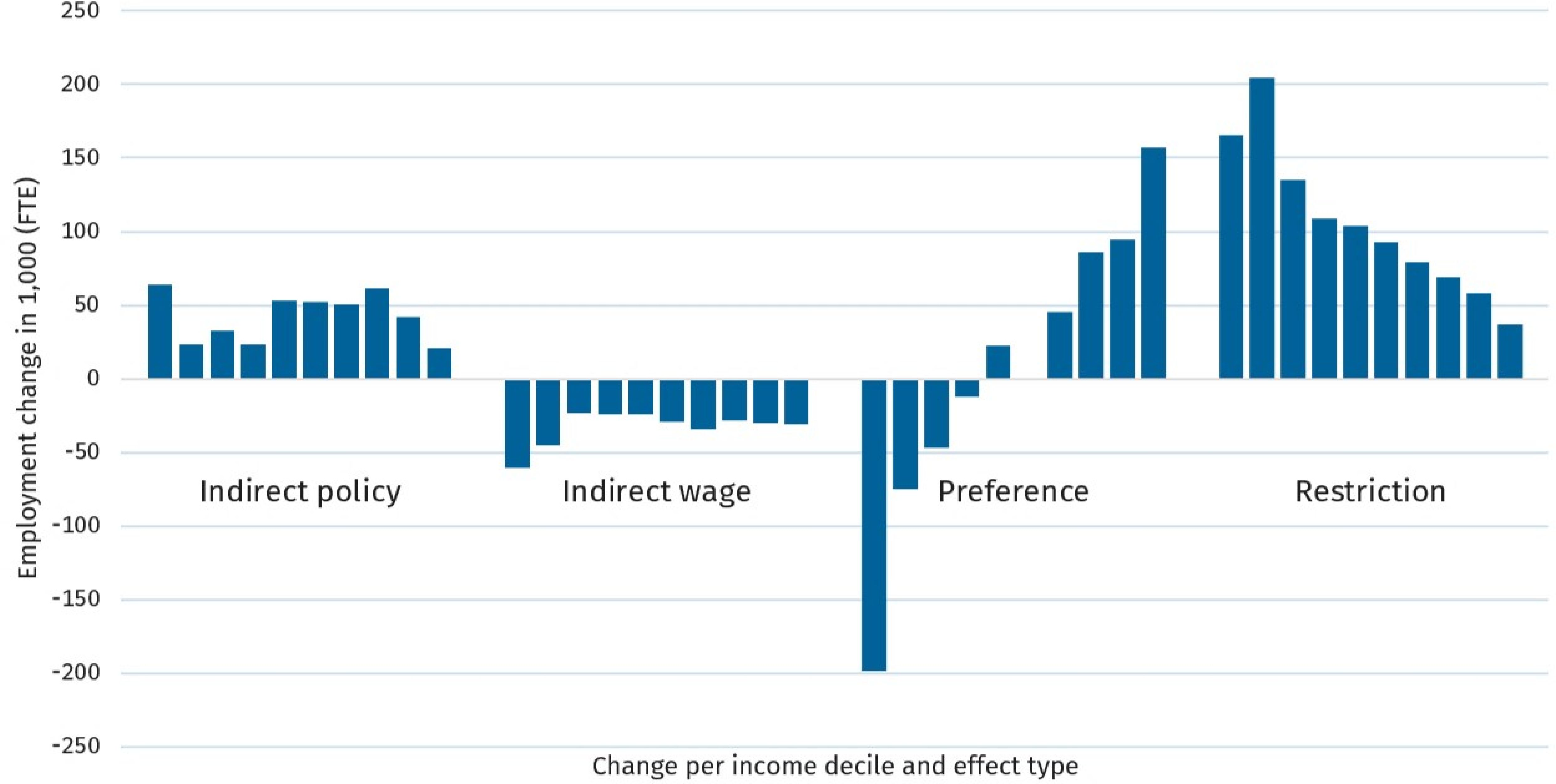
**Figure 4.** Simulated employment changes per income decile and effect type. Note: The columns represent the employment change per households’ disposable income decile from first (left) to tenth (right) decile. Source: IAB-MSM; author’s own presentation.

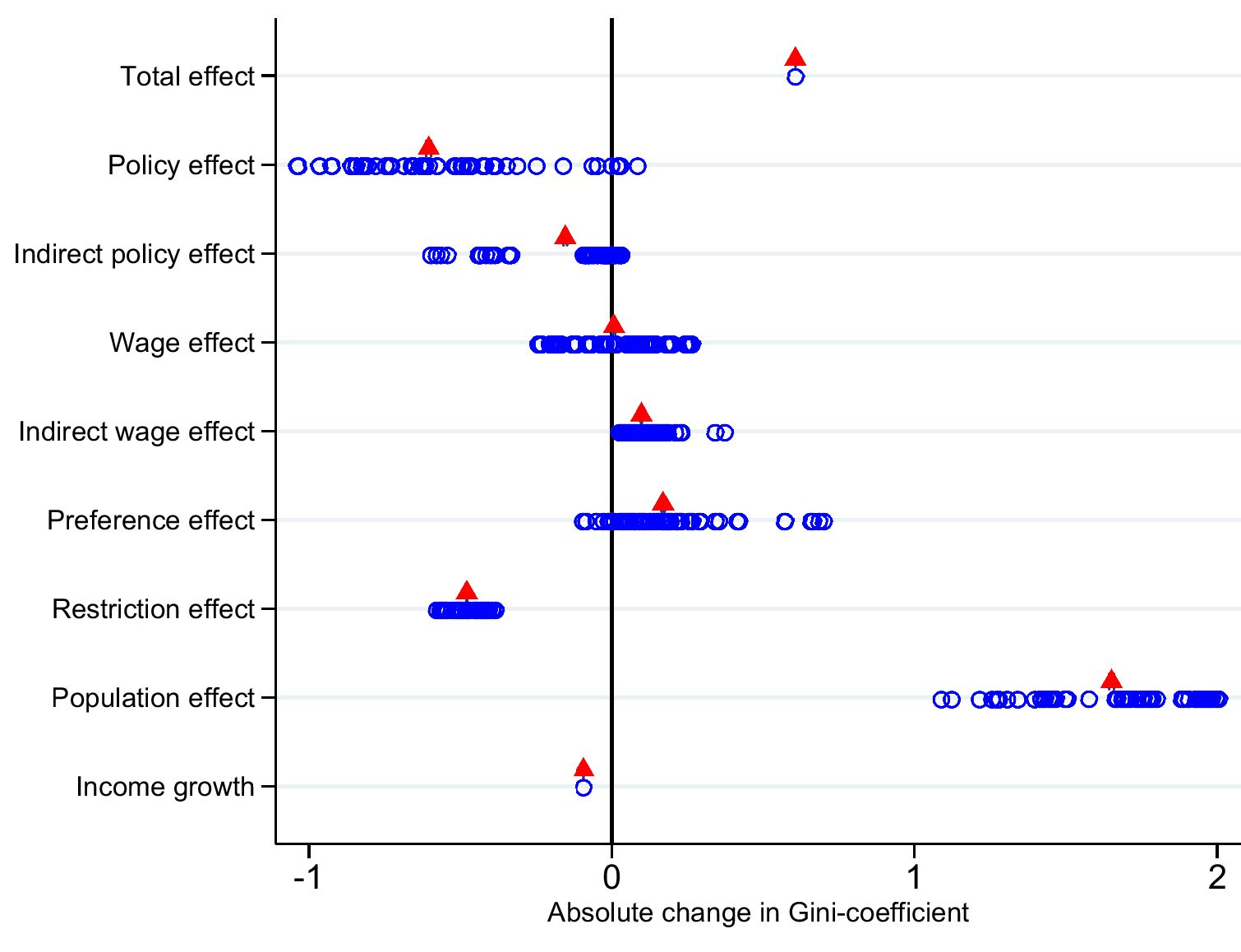
**Figure 5.** Decomposition of change in Gini-coefficient. Note: The triangles mark the Shorrocks-Shapley Value of each effect. Each circle represents one different decomposition.Source: IAB-MSM; author’s own presentation.

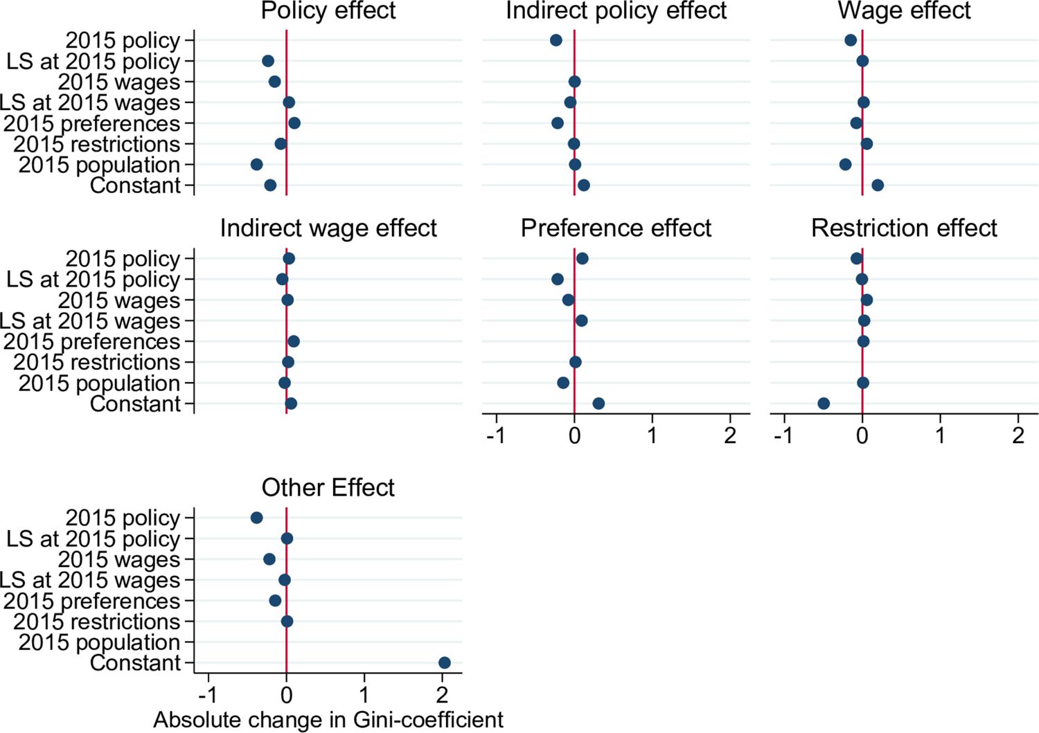
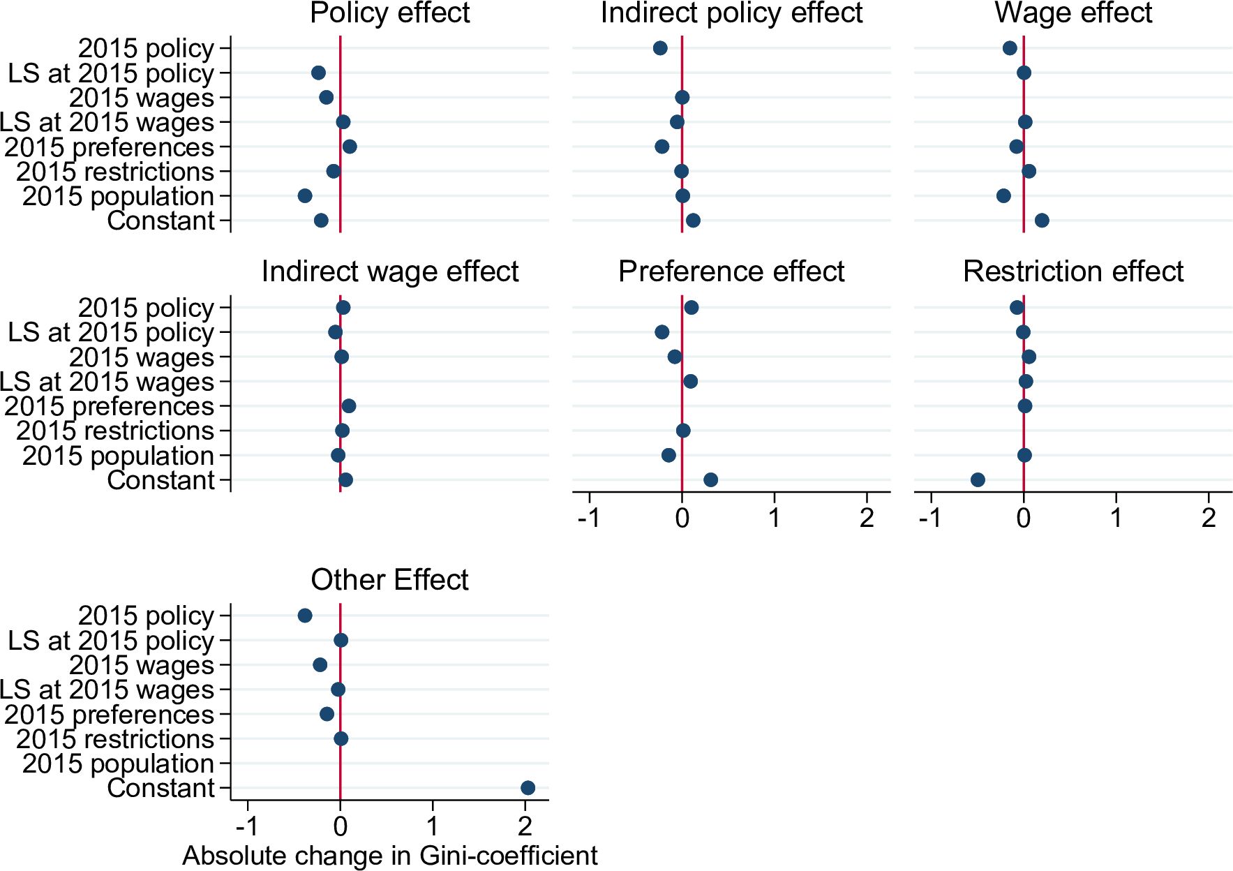
**Figure 6.** Effect heterogeneity. Note: The effect changes are estimated on all 64 possible counterfactual distributions. The constant describes the average effect size when measured at the base period situation.Source: IAB-MSM; author’s own presentation.

Tables

Table 1. Simulated employment changes per working hour category

Employment change in 1000		Working hour category							FTE
Partial effect		0	10	15	20	30	40	50	FTE
Base period	Men	2,073	42	26	125	281	11,312	2,105	14,237
	Women	5,375	1,228	664	2,203	2,074	6,581	561	10,496
	Total	7,448	1,270	690	2,328	2,355	17,893	2,667	24,734
Indirect policy	Men	$-$ −175	$-$ −18	−1	−5	−3	+126	+75	+210
	Women	$-$ −186	$-$ −56	$-$ −20	$-$ −3	+35	+198	+33	+242
	Total	$-$ −361	$-$ −74	$-$ −21	$-$ −8	+32	+324	+107	+452
Indirect wage	Men	+124	+11	+6	+8	+2	−84	−66	−156
	Women	+154	+26	+12	$-$ −10	$-$ −34	$-$ −121	$-$ −26	$-$ −174
	Total	+278	+36	+18	−2	−32	−206	−92	−330
Preference	Men	+156	+32	+27	+46	+115	−480	+105	$-$ −223
	Women	$-$ −490	$-$ −12	+15	+155	+749	−703	+285	+296
	Total	$-$ −334	+20	+43	+201	+864	−1183	+390	+73
Restriction	Men	$-$ −789	+22	+22	+35	+60	+574	+75	+744
	Women	$-$ −431	+42	+34	+90	+125	+130	+10	+304
	Total	$-$ −1220	+65	+56	+126	+186	+704	+84	+1049
Population	Men	+66	−20	−12	−41	−91	−320	+106	$-$ −286
	Women	−655	−269	+26	−361	+146	+873	+99	+869
	Total	−589	−289	+14	−402	+56	+553	+204	+582
Total changes	Men	$-$ −617	+27	+42	+43	+84	−185	+294	+289
	Women	−1,609	−269	+67	−128	+1,022	+377	+400	+1,537
	Total	−2,226	−242	+109	$-$ −85	+1,105	+192	+694	+1,826

Note: FTE = Full-time equivalent.

Source: IAB-MSM; author’s own calculation.

Table 2. Population changes

	2004	2015
Household characteristics
Household type
Singles	39.69%	46.39%
Single parents	9.20%	10.05%
Couples without children	28.42%	27.06%
Couples with children	22.70%	16.50%
Household size
1 person	38.30%	41.88%
2 persons	33.81%	34.05%
3 persons	14.38%	13.97%
4 persons	9.98%	7.73%
5 or more persons	3.53%	2.37%
Individual characteristics
Age
0 - 16 years	17.50%	15.34%
17 - 65 years	63.42%	62.62%
> 65 years	19.08%	22.04%
Nationality (of adults)
German	92.40%	90.90%
Other	7.60%	9.10%
Educational degree (25 - 65 years)
Low degree	37.25%	25.66%
Medium degree	39.78%	43.50%
High degree	22.97%	30.84%
Vocational degree (25 - 65 years)
Vocational degree	86.28%	85.85%
No vocational degree	13.72%	14.15%
Employment status (25 - 65 years)
Blue collar	23.36%	17.92%
White collar	35.66%	48.42%
Self-employed	6.56%	6.03%
Civil servant	4.45%	4.81%
Not employed	29.29%	21.58%
Other	0.68%	1.24%

IAB-MSM = author’s own calculation;

Note: Population shares after household selection with adjusted SOEP weights.

Table 3. Decomposition results: Percentage change in inequality of gross household income from employment

Inequality change
Partial effect	Gini	Atkinson	P90/P10	P90/P50	P50/P10
Indirect policy	-1.14%	-1.27%	-2.81%	-0.64%	-1.95%
Wage	+2.56%	+7.47%	+7.79%	+2.64%	+4.72%
Indirect wage	+1.27%	+0.61%	+1.27%	+0.32%	+0.86%
Preference	+0.76%	+5.73%	+8.95%	+2.14%	+6.38%
Restriction	-4.33%	-0.22%	-0.27%	-0.39%	+0.11%
Population	+2.89%	+5.21%	+3.94%	+5.18%	-1.31%
Total employment	-3.44%	+4.85%	+7.14%	1.43%	+5.40%
Total change	+2.01%	+17.52%	+18.88%	+9.25%	+8.81%

Note: Inflexible households are excluded. For Atkinson and percentile ratios households without income from employment are excluded.

The five columns present the Shorrock-Shapley value of the change in inequality measured with the Gini-coefficient, the Atkinson-index with inequality aversion parameter ∈ = 0.5, and the ratios between the 90th and 10th, the 90th and 50th, and the 50th and 10th income percentiles in percent.

Source: IAB-MSM; author’s own calculation.

Table 4. Decomposition results: Percentage change in inequality of disposable household income

Inequality change
Partial effect	Gini	Atkinson	P90/P10	P90/P50	P50/P10
Policy	-2.30%	-2.91%	-3.33%	-2.39%	-1.07%
Indirect policy	-0.57%	-1.46%	-0.47%	+0.01%	-0.47%
Wage	+0.04%	+0.16%	+0.00%	+0.00%	+0.00%
Indirect wage	+0.38%	+0.65%	-0.06%	-0.01%	-0.05%
Preference	+0.65	+0.32%	-1.42%	-0.01%	-1.41%
Restriction	-1.84%	-3.72%	+0.10%	-0.02%	+0.11%
Population	+6.31%	+6.47%	+8.27%	+4.66%	+3.80%
Growth	-0.34%	-0.97%	-4.70%	-0.47%	-4.25%
Total employment	-1.38%	-4.21%	-1.85%	-0.03%	-1.81%
Total change	+2.33%	-1.46%	-1.62%	+1.78%	-3.34%

Note: The five columns present the Shorrock-Shapley value of the change in inequality measured with the Gini-coefficient, the Atkinson-index with inequality aversion parameter ∈ = 0.5, and the ratios between the 90th and 10th, the 90th and 50th, and the 50th and 10th income percentiles.

Source: IAB-MSM; author’s own calculation.

Table A1. Household selection

Selection step	2004		2015
	N	$\Delta$	N	$\Delta$
Initial number of private households in GSOEP	11,795	(-)	15,996	(-)
Exclusion of households without interviewed head of HH and/or partner	11,721	74	15,952	44
Exclusion of couple households with survey non-response of partner	11,067	654	14,051	2,126
Households interviewed in the simulation year and the following year	9,905	1,162	11,614	1,433
Exclusion of households with missing information on worked hours, wages and other income variables	9,112	972	8,949	3,972
Excluded households	728		1,945
Households considered for income simulation	9,112		10,594
Households considered for inequality analysis	11,067		14,051

Note: N = remaining number of households, $\Delta$ = change in numbers of households in the respective selection step. Exclusions are overestimated, if one simply counts the households affected by a certain condition, since households may be affected more than once.

Source: IAB-MSM; author’s own presentation.

Table A2. Components of net household income in the IAB-MSM

Model stage		Income components	Determined in tax and transfer module?
1		Earned income	no
	+	Self-employed income	no
	+	Capital income	no
	+	Rental income	no
	+	Other income sources (pensions)	no
2	-	Social security contributions	yes
	-	Income tax	yes
	-	Alimony payments	yes
3	+	Child benefit	yes
	+	Child-raising allowance	yes
	+	Unemployment benefits	yes
	+	Federal student support, stipends, claims to maintenance, widow’s allowance, maternity allowance, reduced hours compensation	no
4	+	Housing allowance	yes
	+	Supplementary child allowance	yes
	+	Social assistance for employable persons (SGB II)	yes
	+	Social assistance for unemployable persons (SGB XII)	yes
	=	Net household income	yes

Table A3. Policy parameter

Policy parameter	2004	αρ2004	2015
Benefits
Unemployment Benefit (share of previous net income)	60% (67%)*		60% (67%)*
Unemployment Assistance (share of previous net income)	53% (57%)*
Social Assistance	291€̂	349€	404€
Unemployment Benefit II			404€
Income tax
Marginal tax burden in 1st progressive zone	16% - 24.05%		14% - 23.97%
Marginal tax burden in 2nd progressive zone	24.05% - 45%		23.97% - 42%
Marginal burden in 1st linear zone	45%		42%
Marginal burden in 2nd linear zone (rich tax)			45%
Basic tax allowance	7,664€	9,187€	8,472€
Lower threshold of 2nd progressive zone	12,739€	15,271€	13, 469€
Lower threshold of 1st linear zone	52,151€	62,515€	52,881€
Lower threshold of 2nd linear zone (rich tax)			250,730€
Social security contributions
Contributions to statutory pension insurance	19.5%		18.7%
Contributions to statutory unemployment insurance	6.5%		3.0%
Contributions to statutory health insurance	14.2%		15.5%
Contributions to statutory long-term care insurance	1.7%		2.6% (2.35%)*
Upper threshold of marginal employment (SSC free jobs)	400€	479€	450€
Upper threshold of contributions to statutory pension insurance	5,150€ (4,350€)̂*	6,173€ (5,214€)̂*	6,700€ (6,150€)̂*
Upper threshold of contributions to statutory unemployment insurance	5,150€ (4,350€)̂*	6,173€ (5,214€)̂*	6,700€ (6,150€)̂*
Upper threshold of contributions to statutory health insurance	3,488€	4,181€	4,125€
Upper threshold of contributions to statutory long-term care insurance	3,488€	4.181€	4,125€

Note: The Table includes only the most important policy parameter. Uprating parameter $\alpha$ is set to 1.1987 according to consumer price inflation between 2004 and 2015.

∗ with children.

∗∗ unweighted average over all federal states.

∗∗∗East Germany.

Source: IAB-MSM; author’s own presentation.

Table A4. Estimation results for wage equation of men in East Germany

	2004		2015
	b	se	b	se
Log hourly wages
Years in education	0.0603 ${}^{***}$	(0.0068)	0.0951 ${}^{***}$	(0.0055)
Full-time	-0.0157 ${}^{*}$	(0.0061)	0.0011	(0.0041)
Part-time	-0.0228 ${}^{**}$	(0.0084)	-0.0060	(0.0062)
Human capital dep.	-0.2667 ${}^{***}$	(0.0627)	-0.0622	(0.0654)
Human capital dep. sq.	0.0691 ${}^{***}$	(0.0209)	-0.0438	(0.0318)
Tenure	0.0116 ${}^{*}$	(0.0048)	0.0198 ${}^{***}$	(0.0039)
Tenure sq.	-0.0180	(0.0121)	-0.0216	(0.0112)
Age	0.1133 ${}^{*}$	(0.0496)	0.0444	(0.0510)
Age sq.	-0.2132	(0.1186)	-0.0576	(0.1219)
Age cub.	0.1496	(0.0920)	0.0065	(0.0931)
Married	0.0812 ${}^{*}$	(0.0382)	0.0693 ${}^{*}$	(0.0319)
Separated	0.1510 ${}^{*}$	(0.0733)	0.0363	(0.0969)
Divorced	0.0744	(0.0478)	0.0561	(0.0484)
Children 0-3	-0.0035	(0.0443)	-0.0413	(0.0386)
Children 4-6	0.0346	(0.0502)	0.0618 ${}^{*}$	(0.0315)
Berlin	0.1924 ${}^{***}$	(0.0401)	0.0841 ${}^{**}$	(0.0326)
Constant	-0.1285	(0.6634)	0.3731	(0.6789)
Selection
Low education	0.4902	(0.6294)	0.6708	(0.5615)
Medium education	0.8935	(0.6048)	0.4006	(0.4904)
High education	-1.1962	(0.6265)	-0.5408	(0.5210)
Vocational degree	1.1709 ${}^{*}$	(0.5873)	0.8428	(0.4529)
University degree	1.6311 ${}^{**}$	(0.5976)	0.4673	(0.4678)
Experience	0.0468 ${}^{*}$	(0.0192)	-0.0093	(0.0139)
Human capital dep.	-1.9419 ${}^{***}$	(0.1342)	-1.5065 ${}^{***}$	(0.1313)
Human capital dep. sq.	0.2821 ${}^{***}$	(0.0338)	0.1424 ${}^{***}$	(0.0327)
Age 26-30	0.3566	(0.2406)	1.0566 ${}^{***}$	(0.2412)
Age 31-35	0.3749	(0.2898)	1.0539 ${}^{***}$	(0.2741)
Age 36-40	0.0762	(0.3671)	1.4974 ${}^{***}$	(0.2935)
Age 41-55	-0.2919	(0.4088)	1.5560 ${}^{***}$	(0.3563)
Age 46-50	-0.3446	(0.5127)	1.5454 ${}^{***}$	(0.3789)
Age 51-55	-0.3164	(0.5918)	1.5913 ${}^{***}$	(0.4496)
Age 56-60	-1.2568	(0.6874)	1.6276 ${}^{**}$	(0.5054)
Age 61-65	-2.1426 ${}^{**}$	(0.8132)	0.4614	(0.5823)
Married	0.0600	(0.1564)	0.2883 ${}^{*}$	(0.1353)
Separated	-0.3616	(0.2619)	-0.3547	(0.2593)
Divorced	-0.3332	(0.2135)	-0.2595	(0.2101)
Children 0-3	0.2660	(0.2056)	0.1530	(0.1789)
Children 4-6	0.3129	(0.2041)	0.0436	(0.1529)
kind16	0.1424	(0.1390)	0.1742	(0.1301)
kind17	0.0792	(0.2264)	-0.2543	(0.2935)
Disability	0.0049	(0.0035)	-0.0069	(0.0035)
Other income	-0.8729 ${}^{***}$	(0.1037)	-0.4768 ${}^{***}$	(0.0610)
Other income sq.	0.8984 ${}^{***}$	(0.1605)	0.2678 ${}^{***}$	(0.0457)
Constant	0.8389	(0.5615)	0.5111	(0.4932)
Rho	-0.4362 ${}^{***}$	(0.1301)	0.1927 ${}^{*}$	(0.0843)
Sigma	-0.9927 ${}^{***}$	(0.0345)	-1.0116 ${}^{***}$	(0.0267)
N	1621		1588
Log-likelihood	-807.4515		-843.6526

∗ p < 0.05, ∗∗ p < 0.01, ∗∗∗ p < 0.001.

Source: IAB-MSM; author’s own presentation.

Table A5. Estimation results for wage equation of men in West Germany

	2004		2015
	b	se	b	se
Log hourly wages
Years in education	0.0516 ${}^{***}$	(0.0082)	0.0824 ${}^{***}$	(0.0062)
Full-time	-0.0045	(0.0023)	-0.0010	(0.0020)
Part-time	-0.0204 ${}^{***}$	(0.0054)	-0.0271 ${}^{***}$	(0.0033)
Human capital dep.	-0.2090 ${}^{***}$	(0.0380)	-0.1243 ${}^{**}$	(0.0396)
Human capital dep. sq.	0.0341	(0.0189)	-0.0002	(0.0224)
Tenure	0.0158 ${}^{***}$	(0.0020)	0.0165 ${}^{***}$	(0.0019)
Tenure sq.	-0.0258 ${}^{***}$	(0.0054)	-0.0131 ${}^{**}$	(0.0049)
German	-0.1633	(0.0895)	0.1170	(0.0706)
Years in edu. x German	0.0144	(0.0082)	-0.0020	(0.0062)
Age	0.0766 ${}^{**}$	(0.0252)	0.0283	(0.0237)
Age sq.	-0.1281 ${}^{*}$	(0.0610)	-0.0137	(0.0570)
Age cub.	0.0806	(0.0477)	-0.0214	(0.0444)
Married	0.0512 ${}^{**}$	(0.0181)	0.0757 ${}^{***}$	(0.0171)
Separated	0.0369	(0.0399)	-0.0251	(0.0399)
Divorced	-0.0340	(0.0304)	0.0618 ${}^{*}$	(0.0253)
Children 0-3	0.0447 ${}^{*}$	(0.0188)	0.0340 ${}^{*}$	(0.0159)
Children 4-6	0.0796 ${}^{***}$	(0.0186)	0.0320 ${}^{*}$	(0.0146)
Constant	0.6172	(0.3467)	0.8913 ${}^{**}$	(0.3218)
Selection
Low education	0.5609 ${}^{**}$	(0.2122)	0.6813 ${}^{***}$	(0.1914)
Medium education	0.4134 ${}^{*}$	(0.2057)	0.0442	(0.1637)
High education	-0.5462 ${}^{**}$	(0.2068)	-0.6239 ${}^{***}$	(0.1869)
Vocational degree	0.7051 ${}^{***}$	(0.1706)	0.7336 ${}^{***}$	(0.1527)
University degree	1.3824 ${}^{***}$	(0.1978)	0.6433 ${}^{***}$	(0.1640)
Experience	0.0302 ${}^{**}$	(0.0101)	0.0121	(0.0074)
Human capital dep.	-1.4975 ${}^{***}$	(0.0888)	-1.0907 ${}^{***}$	(0.0744)
Human capital dep. sq.	0.1654 ${}^{***}$	(0.0246)	0.0543 ${}^{**}$	(0.0210)
Age 26-30	0.3408 ${}^{*}$	(0.1358)	0.3479 ${}^{**}$	(0.1181)
Age 31-35	0.5568 ${}^{**}$	(0.1722)	0.7908 ${}^{***}$	(0.1389)
Age 36-40	0.7194 ${}^{***}$	(0.1937)	0.7753 ${}^{***}$	(0.1624)
Age 41-45	0.5321 ${}^{*}$	(0.2516)	0.7208 ${}^{***}$	(0.1887)
Age 46-50	0.3618	(0.2857)	0.7677 ${}^{***}$	(0.2094)
Age 51-55	0.0793	(0.3233)	0.8887 ${}^{***}$	(0.2432)
Age 56-60	-0.5898	(0.3684)	0.3145	(0.2805)
Age 61-65	-1.6890 ${}^{***}$	(0.4238)	-0.6393 ${}^{*}$	(0.3148)
Married	0.0462	(0.1074)	0.2685 ${}^{**}$	(0.0853)
Separated	0.0636	(0.2106)	0.0794	(0.1974)
Divorced	-0.2688	(0.1496)	0.1803	(0.1256)
Children 0-3	0.3631 ${}^{*}$	(0.1471)	-0.1461	(0.0924)
Children 4-6	0.1316	(0.1381)	0.0574	(0.0886)
kind16	-0.0639	(0.0828)	0.1688 ${}^{*}$	(0.0703)
kind17	0.0076	(0.1635)	0.0538	(0.1412)
Disability	-0.0046 ${}^{*}$	(0.0019)	-0.0058 ${}^{***}$	(0.0016)
Other income	-0.3942 ${}^{***}$	(0.0286)	-0.5168 ${}^{***}$	(0.0509)
Other income sq.	0.0869 ${}^{***}$	(0.0066)	0.2913 ${}^{***}$	(0.0769)
Constant	0.6765 ${}^{***}$	(0.1891)	0.8362 ${}^{***}$	(0.1782)
Rho	-0.1286	(0.0693)	0.0578	(0.0559)
Sigma	-1.1161 ${}^{***}$	(0.0157)	-1.0366 ${}^{***}$	(0.0165)
N	4440		5674
Log-likelihood	-1.93e+03		-3.03e+03

∗ p < 0.05, ∗∗ p < 0.01, ∗∗∗ p < 0.001.

Source: IAB-MSM; author’s own presentation.

Table A6. Estimation results for wage equation of women in East Germany

	2004		2015
	b	se	b	se
Log hourly wages
Years in education	0.0776 ${}^{***}$	(0.0055)	0.0816 ${}^{***}$	(0.0044)
Full-time	-0.0062	(0.0046)	0.0043	(0.0030)
Part-time	-0.0116 ${}^{*}$	(0.0053)	-0.0002	(0.0033)
Human capital dep.	-0.1117	(0.0570)	-0.0861	(0.0486)
Human capital dep. sq.	0.0041	(0.0171)	-0.0000	(0.0179)
Tenure	0.0266 ${}^{***}$	(0.0049)	0.0151 ${}^{***}$	(0.0036)
Tenure sq.	-0.0330 ${}^{*}$	(0.0133)	-0.0046	(0.0094)
Age	0.0325	(0.0498)	0.0942 ${}^{*}$	(0.0437)
Age sq.	-0.0074	(0.1241)	-0.1803	(0.1032)
Age cub.	-0.0323	(0.0990)	0.1053	(0.0785)
Married	0.0314	(0.0324)	0.0153	(0.0236)
Separated	-0.0125	(0.0838)	0.0293	(0.0519)
Divorced	-0.0790	(0.0450)	0.0311	(0.0341)
Children 0-3	0.0754	(0.0630)	0.1327 ${}^{**}$	(0.0470)
Children 4-6	0.1813 ${}^{***}$	(0.0472)	0.0507	(0.0313)
Berlin	0.1605 ${}^{***}$	(0.0357)	0.1279 ${}^{***}$	(0.0242)
Constant	0.3610	(0.6300)	-0.2300	(0.5868)
Selection
Low education	6.2022	(.)	1.0227 ${}^{*}$	(0.4361)
Medium education	6.8002 ${}^{***}$	(0.3552)	-0.0080	(0.4148)
High education	6.0726 ${}^{***}$	(0.3613)	-0.5879	(0.4379)
Vocational degree	7.3540 ${}^{***}$	(0.2934)	0.6630	(0.3758)
University degree	7.4677 ${}^{***}$	(0.3056)	0.7411	(0.3820)
Experience	0.0340 ${}^{*}$	(0.0144)	0.0434 ${}^{***}$	(0.0101)
Human capital dep.	-1.2067 ${}^{***}$	(0.1292)	-0.8093 ${}^{***}$	(0.1110)
Human capital dep. sq.	0.0661	(0.0352)	0.0066	(0.0264)
Age 26-30	0.3526	(0.1868)	0.3127	(0.2054)
Age 31-35	0.6714 ${}^{**}$	(0.2449)	0.7782 ${}^{***}$	(0.2280)
Age 36-40	0.5558	(0.2955)	0.5030 ${}^{*}$	(0.2469)
Age 41-45	0.4479	(0.3256)	0.7872 ${}^{**}$	(0.2815)
Age 46-50	0.2952	(0.4109)	0.0829	(0.2946)
Age 51-55	0.0616	(0.4571)	0.1606	(0.3385)
Age 56-60	-0.2991	(0.5244)	-0.4119	(0.3885)
Age 61-65	-1.7425 ${}^{**}$	(0.6272)	-1.8400 ${}^{***}$	(0.4396)
Married	0.2471	(0.1456)	0.3586 ${}^{***}$	(0.1065)
Separated	-0.0537	(0.3317)	0.5252 ${}^{*}$	(0.2443)
Divorced	-0.1005	(0.2036)	0.0039	(0.1545)
Children 0-3	-0.4611 ${}^{*}$	(0.1800)	-0.6359 ${}^{***}$	(0.1314)
Children 4-6	0.7355 ${}^{***}$	(0.1640)	0.5462 ${}^{***}$	(0.1309)
Children 7-16	0.2113	(0.1305)	0.2881 ${}^{**}$	(0.1075)
Children 17-18	0.0907	(0.1894)	0.1543	(0.2345)
Disability	-0.0046	(0.0037)	-0.0091 ${}^{**}$	(0.0028)
Other income	-0.6274 ${}^{***}$	(0.0921)	-0.5656 ${}^{***}$	(0.0694)
Other income sq.	0.6135 ${}^{***}$	(0.1433)	0.4503 ${}^{***}$	(0.0966)
Constant	-5.9186 ${}^{***}$	(0.3300)	0.4937	(0.3798)
Rho	-0.0159	(0.1403)	0.0038	(0.0921)
Sigma	-1.0508 ${}^{***}$	(0.0291)	-1.0927 ${}^{***}$	(0.0304)
N	1831		2025
Log-likelihood	-845.8183		-1.01e+03

* p < 0.05, ∗∗ p < 0.01, ∗∗∗ p < 0.001.

Source: IAB-MSM; author’s own presentation.

Table A7. Estimation results for wage equation of women in West Germany

	2004		2015
	b	se	b	se
Log hourly wages
Years in education	0.0748 ${}^{***}$	(0.0086)	0.0759 ${}^{***}$	(0.0068)
Full-time	0.0032	(0.0017)	0.0023	(0.0013)
Part-time	-0.0044	(0.0023)	-0.0051 ${}^{**}$	(0.0016)
Human capital dep.	-0.0325	(0.0245)	-0.0495 ${}^{**}$	(0.0191)
Human capital dep. sq.	-0.0005	(0.0087)	0.0015	(0.0064)
Tenure	0.0190 ${}^{***}$	(0.0025)	0.0248 ${}^{***}$	(0.0019)
Tenure sq.	-0.0241 ${}^{**}$	(0.0074)	-0.0323 ${}^{***}$	(0.0054)
German	0.0402	(0.0983)	0.0571	(0.0863)
Years in edu. x German	-0.0016	(0.0090)	0.0017	(0.0071)
Age	0.0243	(0.0283)	0.0502 ${}^{*}$	(0.0231)
Age sq.	0.0042	(0.0703)	-0.0770	(0.0550)
Age cub.	-0.0443	(0.0560)	0.0314	(0.0425)
Married	-0.0285	(0.0198)	-0.0277	(0.0152)
Separated	-0.0222	(0.0437)	-0.0155	(0.0328)
Divorced	0.0309	(0.0257)	-0.0379 ${}^{*}$	(0.0190)
Children 0-3	0.1029	(0.0549)	0.0688 ${}^{*}$	(0.0312)
Children 4-6	0.0208	(0.0342)	0.0695 ${}^{***}$	(0.0201)
Constant	0.7980 ${}^{*}$	(0.3768)	0.5628	(0.3134)
Selection
Low education	0.5297 ${}^{**}$	(0.1804)	0.2108	(0.1681)
Medium education	0.4186 ${}^{*}$	(0.1849)	0.2049	(0.1613)
High education	-0.7122 ${}^{***}$	(0.2003)	-0.2802	(0.1752)
Vocational degree	0.7217 ${}^{***}$	(0.1611)	0.7066 ${}^{***}$	(0.1493)
University degree	0.9938 ${}^{***}$	(0.1712)	0.8390 ${}^{***}$	(0.1536)
Experience	0.0042	(0.0049)	0.0016	(0.0038)
Human capital dep.	-0.6856 ${}^{***}$	(0.0596)	-0.2717 ${}^{***}$	(0.0478)
Human capital dep. sq.	-0.0253	(0.0134)	-0.0944 ${}^{***}$	(0.0113)
Age 26-30	0.6996 ${}^{***}$	(0.1126)	0.3663 ${}^{***}$	(0.0934)
Age 31-35	0.9727 ${}^{***}$	(0.1226)	0.7185 ${}^{***}$	(0.1020)
Age 36-40	1.0663 ${}^{***}$	(0.1299)	0.8993 ${}^{***}$	(0.1099)
Age 41-45	1.0626 ${}^{***}$	(0.1443)	1.1341 ${}^{***}$	(0.1146)
Age 46-50	0.9881 ${}^{***}$	(0.1550)	1.1266 ${}^{***}$	(0.1224)
Age 51-55	0.7691 ${}^{***}$	(0.1673)	1.0450 ${}^{***}$	(0.1322)
Age 56-60	0.6069 ${}^{***}$	(0.1794)	0.8570 ${}^{***}$	(0.1478)
Age 61-65	-0.4658 ${}^{*}$	(0.2170)	0.0948	(0.1695)
Married	0.1655 ${}^{*}$	(0.0789)	-0.0021	(0.0570)
Separated	-0.0561	(0.1660)	-0.1495	(0.1205)
Divorced	0.0004	(0.1039)	-0.0265	(0.0743)
Children 0-3	-1.2915 ${}^{***}$	(0.1023)	-0.9322 ${}^{***}$	(0.0664)
Children 4-6	0.2875 ${}^{**}$	(0.0877)	0.3254 ${}^{***}$	(0.0614)
Children 7-16	0.1757 ${}^{**}$	(0.0678)	0.1959 ${}^{***}$	(0.0481)
Children 17-18	0.0045	(0.1277)	-0.1579	(0.0822)
Disability	-0.0087 ${}^{***}$	(0.0019)	-0.0085 ${}^{***}$	(0.0012)
Other income	-0.1455 ${}^{***}$	(0.0184)	-0.2526 ${}^{***}$	(0.0236)
Other income sq.	0.0160 ${}^{***}$	(0.0021)	0.1365 ${}^{***}$	(0.0234)
Constant	0.0767	(0.1681)	0.1098	(0.1603)
Rho	-0.0639	(0.0879)	0.0917	(0.0695)
Sigma	-1.0406 ${}^{***}$	(0.0215)	-1.0411 ${}^{***}$	(0.0151)
N	5078		7259
Log-likelohood	-2.73e+03		-4.47e+03

∗ p < 0.05, ∗∗ p < 0.01, ∗∗∗ p < 0.001.

Source: IAB-MSM; author’s own presentation.

Table A8. Estimation results for the unemployment probabilities

	2004		2015
	Women	Men	Women	Men
Regional unemployment rate	0.0593 ${}^{***}$	0.0320 ${}^{***}$	0.0822 ${}^{***}$	0.0616 ${}^{***}$
	(0.0079)	(0.0063)	(0.0140)	(0.0136)
Age	-0.0740 ${}^{***}$	0.0025	-0.0783 ${}^{***}$	-0.0527 ${}^{***}$
	(0.0062)	(0.0073)	(0.0069)	(0.0082)
Age sq.	0.0008 ${}^{***}$	0.0000	0.0008 ${}^{***}$	0.0007 ${}^{***}$
	(0.0001)	(0.0001)	(0.0001)	(0.0001)
Nationality
German	Reference
OECD	0.2640	0.0643	0.1651	-0.2239
	(0.1917)	(0.1842)	(0.1697)	(0.2154)
Other	0.3403	0.2539	0.3372 ${}^{**}$	-0.0879
	(0.1737)	(0.1625)	(0.1060)	(0.1513)
Educational degree
Low degree	Reference
Medium degree	-0.2089 ${}^{*}$	-0.2914 ${}^{***}$	-0.2340 ${}^{**}$	-0.2797 ${}^{**}$
	(0.0917)	(0.0835)	(0.0824)	(0.0894)
High degree	-0.5648 ${}^{***}$	-0.8269 ${}^{***}$	-0.4637 ${}^{***}$	-0.4932 ${}^{***}$
	(0.1348)	(0.1283)	(0.1107)	(0.1166)
No vocational degree	0.1027	0.1806	0.2892 ${}^{***}$	0.2042
	(0.1002)	(0.1414)	(0.0846)	(0.1060)
Previous employment
Employed in t-1	-1.2011 ${}^{***}$	-1.8202 ${}^{***}$	-0.4772 ${}^{**}$	-1.3053 ${}^{***}$
	(0.1714)	(0.1030)	(0.1663)	(0.2121)
Employed in t-2	0.0593	-0.1668	-0.5057 ${}^{**}$	-0.2350
	(0.1621)	(0.1108)	(0.1766)	(0.1904)
Employed in t-3	0.0480	-0.3755 ${}^{***}$	-0.0785	-0.0751
	(0.1191)	(0.1075)	(0.1741)	(0.1368)
$N$	3446	3659	4288	4108
Pseudolikelihood	-788.5288	-536.3061	-787.5285	-563.0143

∗ p < 0.05, ∗∗ p < 0.01, ∗∗∗ p < 0.001.

Note: t statistics in parentheses.

Source: IAB-MSM; author’s own presentation.

Table A9. Estimation results for the labor supply preferences of single men

	2004		2015
	Coef.	s.e.	Coef.	s.e.
Consumption	-0.6219	(1.4808)	7.9233 ${}^{**}$	(2.8858)
Consumption sq.	-0.04069	(0.0555)	0.1869 ${}^{**}$	(0.0707)
Consumption x Leisure	0.09482	(0.3565)	-1.4357 ${}^{*}$	(0.7193)
Leisure	92.545 ${}^{***}$	(11.0540)	85.453 ${}^{***}$	(10.1909)
Leisure sq.	-12.247 ${}^{***}$	(1.4535)	-9.8510 ${}^{***}$	(1.3204)
Leisure x
High education	-0.6056	(0.5755)	-0.4818	(0.4998)
Low education	1.8243 ${}^{**}$	(0.5659)	0.5176	(0.4642)
East Germany	1.3023 ${}^{**}$	(0.4798)	0.2647	(0.3847)
German nationality	0.3709	(1.1765)	0.5161	(0.4825)
Age	-0.6355	(1.7146)	-3.9675 ${}^{***}$	(1.0906)
Age sq.	12.437	(20.4404)	48.661 ${}^{***}$	(12.6555)
Fixed costs of work	3.9099 ${}^{***}$	(0.6724)	3.5089 ${}^{***}$	(0.4943)
Fixed costs of full-time	-3.1132 ${}^{***}$	(0.3355)	-3.2498 ${}^{***}$	(0.3006)
N	602		724
Log-likelihood	-502.42		-675.89
$U_{C}§lt;0$	0.9668		0.02999

∗ p < 0.05, ∗∗ p < 0.01, ∗∗∗ p < 0.001 .

Source: IAB-MSM; author’s own presentation.

Table A10. Estimation results for the labor supply preferences of single women

	2004		2015
	Coef.	s.e.	Coef.	s.e.
Consumption	0.5100	(0.8057)	3.2805 ${}^{*}$	(1.5159)
Consumption sq.	0.1637 ${}^{**}$	(0.0568)	0.2923 ${}^{*}$	(0.1191)
Consumption x Leisure	0.1027	(0.1974)	-0.08498	(0.3837)
Leisure	113.22 ${}^{***}$	(8.8914)	89.797 ${}^{***}$	(6.4361)
Leisure sq.	-13.687 ${}^{***}$	(1.0840)	-11.075 ${}^{***}$	(0.8002)
Leisure x
High education	-0.9524	(0.5770)	-0.4796	(0.3976)
Low education	0.5652	(0.5740)	0.8085	(0.4143)
East Germany	0.3233	(0.5053)	0.2691	(0.3548)
German nationality	0.9445	(0.9306)	-1.1898 ${}^{**}$	(0.4508)
Age	-5.1194 ${}^{***}$	(1.4995)	-2.0370	(1.0574)
Age sq.	74.421 ${}^{***}$	(17.8229)	34.874 ${}^{**}$	(11.9136)
Fixed costs of work	2.8597 ${}^{***}$	(0.4106)	3.2088 ${}^{***}$	(0.2792)
Fixed costs of full-time	-2.4068 ${}^{***}$	(0.2324)	-1.4462 ${}^{***}$	(0.1557)
N	525		862
Log-likelihood	-564.09		-1125.8
$U_{C}§lt;0$	0.03401		0.01226

∗ p < 0.05, ∗∗ p < 0.01, ∗∗∗ p < 0.001.

Source: IAB-MSM; author’s own presentation.

Table A11. Estimation results for the labor supply preferences of single parents

	2004		2015
	Coef.	s.e.	Coef.	s.e.
Consumption	-0.4519	(1.5239)	0.1529	(3.5820)
Consumption sq.	0.08838	(0.3872)	0.2725 ${}^{**}$	(0.0987)
Consumption x Leisure	0.4187	(0.3614)	0.3794	(0.9028)
Leisure	103.88 ${}^{***}$	(12.4890)	111.48 ${}^{***}$	(10.3108)
Leisure sq.	-13.111 ${}^{***}$	(1.3576)	-13.358 ${}^{***}$	(1.1540)
Leisure x
East Germany	-1.6070 ${}^{**}$	(0.6184)	-1.3669 ${}^{**}$	(0.4225)
German nationality	2.0888 ${}^{*}$	(0.9744)	0.04071	(0.6061)
High education	0.1565	(0.8211)	-1.1287 ${}^{*}$	(0.5198)
Low education	2.2245 ${}^{***}$	(0.6427)	1.4929 ${}^{**}$	(0.4592)
Age	-2.3404	(3.2685)	-3.6618	(2.1359)
Age sq.	25.516	(41.0984)	43.342	(25.2813)
Children 0-3	4.9634 ${}^{***}$	(1.1028)	3.8055 ${}^{***}$	(0.7702)
Children 4-6	2.8139 ${}^{***}$	(0.6554)	1.4972 ${}^{**}$	(0.4876)
Children 7-16	0.6357	(0.3874)	0.6774 ${}^{*}$	(0.3138)
Children >16	1.3024 ${}^{*}$	(0.5400)	0.6987	(0.5192)
Fixed costs of work	2.8658 ${}^{***}$	(0.3697)	2.6273 ${}^{***}$	(0.2451)
Fixed costs of full-time	-1.2038 ${}^{***}$	(0.2668)	-0.9790 ${}^{***}$	(0.1860)
N	299		634
Log-likelihood	-445.12		-999.52
$U_{C}§lt;0$	0.004300		0.0004507

∗ p < 0.05, ∗∗ p < 0.01, ∗∗∗ p < 0.001.

Source: IAB-MSM; author’s own presentation.

Table A12. Estimation results for the labor supply preferences of couples where only one spouse is flexible

	2004		2015
	Coef.	s.e.	Coef.	s.e.
Consumption	0.6217	(1.4490)	7.9105 ${}^{***}$	(1.6243)
Consumption sq.	0.4029 ${}^{***}$	(0.0702)	0.4141 ${}^{***}$	(0.0694)
Consumption x Leisure	0.3898	(0.3162)	-1.0822 ${}^{**}$	(0.3507)
Leisure	84.463 ${}^{***}$	(5.9911)	84.997 ${}^{***}$	(5.6047)
Leisure sq.	-10.587 ${}^{***}$	(0.7109)	-10.476 ${}^{***}$	(0.6454)
Leisure x
Woman	5.9726 ${}^{***}$	(0.5172)	4.7809 ${}^{***}$	(0.4087)
Leisure of spouse	0.4631 ${}^{*}$	(0.2316)	0.4475	(0.2367)
East Germany	1.1401	(0.6794)	0.3378	(0.5699)
East Germany - Woman	-2.9637 ${}^{***}$	(0.7627)	-1.4917 ${}^{*}$	(0.6606)
German nationality	-1.1034 ${}^{*}$	(0.5468)	-0.7173	(0.4119)
High education - Woman	-1.1636 ${}^{**}$	(0.3744)	-0.6819 ${}^{*}$	(0.3201)
High education - Man	-0.05177	(0.3317)	0.06458	(0.3113)
Low education - Woman	1.0177 ${}^{*}$	(0.4058)	0.5498	(0.3899)
Low education - Man	-0.3108	(0.4779)	0.2260	(0.4211)
Age	-4.4804 ${}^{***}$	(1.2896)	-3.6811 ${}^{***}$	(1.0843)
Age sq.	63.590 ${}^{***}$	(14.8757)	52.129 ${}^{***}$	(11.9375)
Children 0-3	4.0337 ${}^{***}$	(0.5750)	2.7117 ${}^{***}$	(0.4410)
Children 4-6	1.5221 ${}^{***}$	(0.4286)	0.9293 ${}^{**}$	(0.3156)
Children 7-16	0.8736 ${}^{***}$	(0.2014)	0.6289 ${}^{***}$	(0.1799)
Children >16	0.5671 ${}^{**}$	(0.2194)	0.3523	(0.2805)
Fixed costs of work	2.6902 ${}^{***}$	(0.2091)	2.7418 ${}^{***}$	(0.1963)
Fixed costs of full-time	-1.7784 ${}^{***}$	(0.1535)	-1.4269 ${}^{***}$	(0.1386)
N	1050		1151
Log-likelihood	-1431.3		-1624.8
$U_{C}§lt;0$	0.001633		0.001862

∗ p < 0.05, ∗∗ p < 0.01, ∗∗∗ p < 0.001.

Source: IAB-MSM; author’s own presentation.

Table A13. Estimation results for the labor supply preferences of couples where both spouses are flexible

	2004		2015
	Coef.	s.e.	Coef.	s.e.
Consumption	1.4838 ${}^{**}$	(0.5294)	12.561 ${}^{***}$	(2.0692)
Consumption sq.	0.1944 ${}^{***}$	(0.0385)	0.3553 ${}^{***}$	(0.0516)
Consumption x Leisure man	0.009652	(0.0925)	-1.0063 ${}^{**}$	(0.3598)
Consumption x Leisure woman	-0.02770	(0.0853)	-1.2710 ${}^{***}$	(0.2936)
Leisure man	94.432 ${}^{***}$	(7.2397)	93.569 ${}^{***}$	(5.7676)
Leisure man sq.	-10.843 ${}^{***}$	(0.9208)	-10.851 ${}^{***}$	(0.6849)
Leisure man x
East Germany	-4.6848	(3.1804)	-2.8742	(2.9422)
German nationality - Man	-0.9338 ${}^{*}$	(0.4397)	-0.6835 ${}^{*}$	(0.3021)
High education - Man	-1.2707 ${}^{***}$	(0.2680)	0.1922	(0.2509)
Low education - Man	0.7592 ${}^{*}$	(0.2948)	0.4963	(0.2573)
Age - Man	-3.7896 ${}^{***}$	(0.9974)	-2.4464 ${}^{**}$	(0.8087)
Age sq. - Man	53.132 ${}^{***}$	(11.3029)	32.686 ${}^{***}$	(9.0016)
Leisure woman	101.64 ${}^{***}$	(4.4523)	91.721 ${}^{***}$	(4.3630)
Leisure woman sq.	-12.132 ${}^{***}$	(0.4732)	-10.546 ${}^{***}$	(0.4320)
Leisure woman x
East Germany	-7.4150 ${}^{*}$	(3.0151)	-5.0222	(2.7395)
German nationality - Woman	-0.3894	(0.3941)	-0.8842 ${}^{***}$	(0.2679)
High education - Woman	-1.2869 ${}^{***}$	(0.2164)	-0.7146 ${}^{***}$	(0.1953)
Low education - Woman	0.1559	(0.2384)	0.6132 ${}^{**}$	(0.2345)
Age - Woman	-2.1765 ${}^{*}$	(0.8896)	-2.0661 ${}^{**}$	(0.7590)
Age sq. - Woman	42.169 ${}^{***}$	(10.6571)	32.285 ${}^{***}$	(8.7851)
Children 0-3	6.9415 ${}^{***}$	(0.3614)	5.0673 ${}^{***}$	(0.2656)
Children 4-6	3.1790 ${}^{***}$	(0.2612)	1.5697 ${}^{***}$	(0.1733)
Children 7-16	1.7139 ${}^{***}$	(0.1183)	1.3189 ${}^{***}$	(0.0999)
Children >16	0.7215 ${}^{***}$	(0.1306)	0.7273 ${}^{***}$	(0.1676)
Leisure man x Leisure woman	-1.0564 ${}^{*}$	(0.4114)	-1.0340 ${}^{*}$	(0.4519)
Leisure man x Leisure woman x
East Germany	1.2956	(0.8144)	0.8652	(0.7362)
German couple	-0.05897	(0.1072)	0.1427 ${}^{*}$	(0.0693)
Fixed costs of work - Man	4.5919 ${}^{***}$	(0.4411)	4.0863 ${}^{***}$	(0.3150)
Fixed costs of work - Woman	2.1989 ${}^{***}$	(0.1077)	2.2333 ${}^{***}$	(0.0979)
Fixed costs of full-time - Man	-3.7534 ${}^{***}$	(0.2227)	-3.0504 ${}^{***}$	(0.1560)
Fixed costs of full-time - Woman	-1.5968 ${}^{***}$	(0.0953)	-0.8672 ${}^{***}$	(0.0869)
N	2879		3154
Log-likelihood	-6504.1		-7677.6
$U_{C}§lt;0$	0.01353		0.002498

∗ p < 0.05, ∗∗ p < 0.01, ∗∗∗ p < 0.001.

Source: IAB-MSM; author’s own presentation.

Table A14. Regression results: Effect heterogeneity

	Policy	I. pol.	Wage	I. wage	Pref.	Restr.	Other
2015 policy		-0.235*** (-9.84)	-0.150*** (-17.56)	0.032** (2.88)	0.102*** (3.85)	-0.072*** (-15.84)	-0.381*** (-24.05)
LS 2015 policy	-0.235*** (-8.96)		0.003 (0.40)	-0.052*** (-4.65)	-0.216*** (-8.09)	-0.005 (-1.11)	0.009 (0.55)
2015 wages	-0.150*** (-5.71)	0.003 (0.14)		0.016 (1.41)	-0.077** (-2.90)	0.057*** (12.49)	-0.217*** (-13.72)
LS 2015 wages	0.032 (1.23)	-0.052* (-2.19)	0.016 (1.85)		0.093*** (3.50)	0.023*** (5.05)	-0.022 (-1.41)
2015 preferences	0.102*** (3.90)	-0.216*** (-9.03)	-0.077*** (-9.07)	0.093*** (8.32)		0.014** (3.03)	-0.144*** (-9.07)
2015 restrictions	-0.072** (-2.76)	-0.005 (-0.21)	0.057*** (6.69)	0.023* (2.05)	0.014 (0.52)		0.009 (0.58)
2015 population	-0.381*** (-14.51)	0.009 (0.37)	-0.217*** (-25.48)	-0.022 (-1.99)	-0.144*** (-5.39)	0.009* (2.02)
Constant	-0.206*** (-5.93)	0.121*** (3.84)	0.197*** (17.49)	0.059*** (3.99)	0.312*** (8.84)	-0.496*** (-82.06)	2.031*** (96.91)
N	64	64	64	64	64	64	64
r2	0.859	0.763	0.950	0.657	0.696	0.887	0.937

∗ p < 0.05, ∗∗ p < 0.01, ∗∗∗ p < 0.001.

Note: t statistics in parentheses.

Source: IAB-MSM; author’s own presentation.