IrpetDin. A Dynamic Microsimulation Model for Italy and the Region of Tuscany
- Istituto Regionale Programmazione Economica della Toscana, Italy
- Article
- Figures and data
- Jump to
Abstract
IrpetDin is a dynamic microsimulation model, developed by IRPET (Regional Institute for Economic Planning of Tuscany) to study the future socio-demographic structure of the population and to evaluate the effects of social security programmes in Italy and in Tuscany over the medium to long-term. The model, based on the Eurostat Survey on Income and Living Conditions, makes projections from 2009 to 2050 and it is organised in modules: demography, education, labour and income and social security. IrpetDin produces realistic projections even for the Region of Tuscany and models education and labour with details. Probabilities and rates are estimated differently for Italy and Tuscany, trough regional administrative data. Education careers are completely simulated, from the choice of secondary school to drop-out, from university enrolment to graduation. Labour supply is endogenously determined while labour demand is driven from IRPET’s macro model. The matching of labour supply and demand is modelled by sector of activity and education, in order to estimate the quantitative and the qualitative mismatch.
1. Introduction
IrpetDin is a dynamic microsimulation model, developed by IRPET (Regional Institute for Economic Planning of Tuscany), able to make future projections regarding the evolution of a representative sample of the Italian and Tuscan population. The model can be used by IRPET to support the regional policy maker, that is the Region of Tuscany, in evaluating the effects of policies and in planning new interventions.
The model analyses the socio-demographic structure of the population and evaluates the effects of social security programmes over the medium to long-term. In the baseline scenario, predictions are based on specific assumptions regarding the future evolution of demographic and economic indicators as well as social security policies. However, IrpetDin also allows for an evaluation of different scenarios by modifying assumptions regarding exogenous variables and by simulating reforms of current social security policies.
IrpetDin is based on EU-SILC 2008, the Eurostat Survey on Income and Living Conditions, which is also representative at regional level. Indeed, the model is designed to produce realistic predictions for Italy and the Region of Tuscany. It simulates demography, education, labour and income and social security, from 2008 to 2050. Predictions have been validated for the 2008-2017 period, in relation to which real data is already available.
With respect to other microsimulation models, we believe IrpetDin to be particularly innovative with regard to its territorial coverage and its ability to model education and labour.
IrpetDin particularly focuses on collecting accurate data for Tuscany. Probabilities and rates are estimated differently for Italy and Tuscany, by exploiting regional administrative data where available. The model therefore requires an extensive range of different data sources, allowing us to obtain realistic estimates even at regional level.
Education is modelled in more detail compared with other microsimulation models, from high-school enrolment to school life, from final results to enrolment in university. If the relative data is available, we also take into account the effects of family background on education outcomes.
Labour is modelled differently compared to many other microsimulation models. We do not estimate the probability of transitions from education to work, but we match labour supply, endogenously determined within IrpetDin, and labour demand, taken from Dante, IRPET’s macro model, by sector and level of education. IrpetDin can therefore predict the future evolution of the unemployment rate and evaluate the “qualitative mismatch” between labour supply and demand.
This paper describes how IrpetDin works, as well as presenting the main results regarding the evolution of the Italian and Tuscan population, in terms of demography, education, labour and social security policies. Section 2 describes the general features, section 3 presents the adjustments made to the initial sample and section 4 deals with the structure of the model. The paper goes on to describe the simulation of events for every module, from demography (section 5) through to social security (section 8). Validation and prediction results are presented in sections 9 and 10. Some final comments about further developments conclude the paper.
2. General features
In this section, we discuss IrpetDin’s general features with regard to its uses, selection of the base dataset, the type of model, ageing method, time modelling, linkage with macro models and the development environment.
As described in Li and O'Donoghue (2013), dynamic microsimulation models may have different uses, with the most common being: i) to project socio-economic development trends under current policies, and ii) to evaluate the future performance and reforms of social security programmes, such as pensions, education, health and long-term care. Andreassen (1993) uses the MOSART model to show the evolution of the population, labour force, levels of education and future costs of state pensions under current legislation in Norway. In their LABORsim model, Leombruni and Richiardi (2006) focus the analysis on education, labour and pensions. Out of all social security programmes, pensions are undoubtedly the most studied. Models such as LIAM (O’Donoghue et al., 2009) and MIDAS (Dekkers, 2010) have been used to look at pension reforms, with a few models also being used to examine changes to funding for education (e.g. Hain and Helberger, 1986).
IrpetDin aims to analyse socio-demographic trends and to evaluate the effects of current social security programmes and their reforms. With respect to other microsimulation models, we model education and labour in greater detail and, consequently, we focus more on analysing future education attainment trends and labour market indicators. With regard to social security programmes, IrpetDin is able to evaluate the effects of pension reforms and analyse the future performance of health and long-term care under current legislation.
Dynamic microsimulation models may use different types of base data: i) administrative data; ii) census data; iii) household survey data; iv) synthetic data. IrpetDin is based on household survey data, namely the European Union Statistics on Income and Living Conditions (EU-SILC). EU-SILC collects extensive information on family members and incomes, even at regional level. It is therefore able to meet IrpetDin’s objective of predicting both socio-demographic trends and the effects of welfare reforms, even only with regard to the Region of Tuscany. However, as is the case with all survey data, the issue with EU-SILC is its small sample size, making it unreliable with regard to certain, specific information and inaccurate in terms of small area estimates. For these reasons, which we will explain in more detail later on, adjustments need to be made to the original EU-SILC sample. Other Italian dynamic microsimulation models have also used EU-SILC, such as Mazzaferro and Morciano (2012) and Caretta et al. (2012). To overcome the issues involved with the survey data, Caretta et al. (2012) individually matched EU-SILC and administrative data.
As is the case for the majority of dynamic microsimulation models, IrpetDin is a population model and a closed model. Indeed, it models a cross-section survey, representing the Italian population, rather than a single cohort, over a defined period of time. Furthermore, the closed model method is used as it presents a fixed set of individuals, with the exception of newborns and migrants, to simulate events, i.e. those belonging to the initial sample. It then uses a dynamic ageing procedure to update the initial sample over time, changing the attributes of the individuals concerned (e.g. their age, employment status, etc.) instead of altering sample weights, as would be the case with a static ageing procedure. These updates are completed annually, as per many discrete-time dynamic models.
Many microsimulation models are somehow linked to macro models, with the aim of reinforcing results for macro indicators, such as the unemployment rate. Nonetheless, only rarely are they fully integrated with macro models, including iterations and feedback effects. They usually just align a number of policy indicators to external macro data. Also IrpetDin aligns certain indicators to exogenous sources including, as we will explain later on, labour demand, aligned to IRPET’s macro model.
3. Adjustment of the initial sample
In EU-SILC 2008, the weighted age structure of the sample is inconsistent with actual data. We therefore need to adjust the distribution of the population by age and by gender, the accuracy of which is crucial for the dynamic microsimulation model. Figure 1a shows the distribution of the Italian population by age in EU-SILC and according to official data by ISTAT, the Italian National Institute of Statistics. As can be easily seen, EU-SILC strongly overestimates the number of people aged 0 and under/overestimates other ages. Furthermore, the initial sample does not specify the age of people over 79 years old. For these reasons, we have adjusted the initial sample by increasing/decreasing individuals’ ages by one or, at the most, two years, until the population by age is as close as possible to actual figures.1 We then randomly attributed precise ages to individuals over 79.

Italian population by age. Italy.
Figure 1b shows the distribution of the adjusted sample compared to actual data. Although some differences still remain, the two curves are more similar compared with the initial sample (Figure 1a).
The second important adjustment refers to labour market indicators. EU-SILC is not designed to describe the labour market in detail. It tends not to be very accurate in its estimates of un/employment rates. On the contrary, the Labour Force Survey (LFS) is used to measure official employment and unemployment rates. Since the aim of IrpetDin is to predict future labour market indicators, we have adjusted the EU-SILC’s initial distribution of individuals by employment status (employed, unemployed, inactive) with respect to LFS, by age class and by gender.
As is the case with all survey data, another issue with EU-SILC concerns sample weights and the creation of new households. For example, to simulate marriage between individuals belonging to different families of origin, the model may create a new household composed of members with different weights. To overcome this problem, we have completed a sort of re-weighting, by repeating each sample individual as many times as is the ratio between his/her sample weight and the minimum sample weight2. In this way, every individual has the same weight, equal to 1.
Finally, EU-SILC does not provide information on the employment history of people who were employed in the initial sample. Given that pension amounts depend on employment contributions paid in the past, we imputed the past incomes of employed individuals, starting from when they first entered the labour market, by assuming the same nominal labour income growth rates for those in the same sector of activity and territory (calculated on the National Accounts provided by ISTAT). We are aware of the limits of this assumption in terms of incomes variability. Indeed, as a future development of the model, we would like to integrate the sample with true administrative data on the work history of the individuals in the sample.
4. Irpetdin’s structure
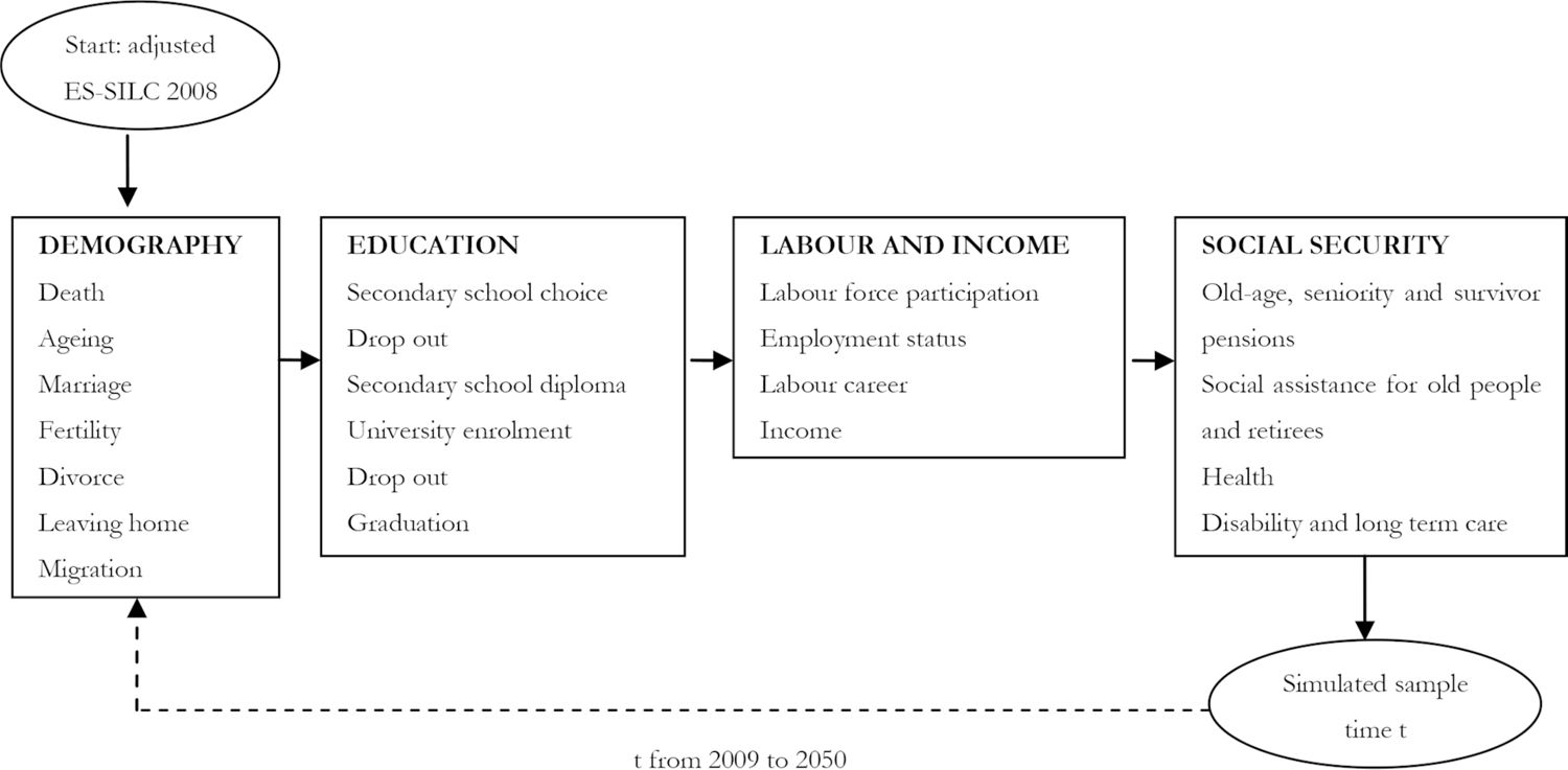
IrpetDin is a classic dynamic microsimulation model, organised in modules (Figure 2). It starts by simulating each module for the adjusted initial sample, referring to 2008.
IrpetDin’s structure.
It simulates demographic events, from ageing to migration, then educational attainment at secondary and tertiary-school level, labour market events, such as entries to the labour force or careers, and, finally, it models social security policies, including pensions, health and long-term care. After the last module, a new sample data set is produced, updated as at 2009, based on which IrpetDin simulates all events for each module for 2010, and so on and so forth until 2050.
IrpetDin events, or, in other words, transitions between states, can be simulated with a probabilistic or deterministic approach. Probabilistic transitions are completed using the so-called Monte Carlo method, whereby a random number is drawn from a uniform distribution [0,1] and attributed to each observation. If the random value is lower than the probability of an event occurring, then the event actually occurs. In IrpetDin, we obtain probabilities in three different ways: i) by estimating econometric models; ii) by calculating specific rates using specific socio-demographic characteristics; or, iii) by taking probabilities estimated by external research institutes. Probabilities refer to data updated as at the base year and do not change over time. Only the characteristics that determine the probabilities/rates are updated over time through dynamic microsimulation. Deterministic events mainly refer to retirement in the social security module, with the exception of ageing.
As mentioned in the introduction, and as we will explain in more detail later on, IrpetDin makes projections based on both specific assumptions regarding the future evolution of demographic indicators and social security policies, as well as by aligning economic variable trends from IRPET’s macro model called “Dante”.
The following sections provide a detailed description of each IrpetDin module. Table A1, attached hereto, presents synthetic information on probability estimation methods, the variables that determine events and data sources for probabilities estimation and for the eventual alignements.
5. Demography
For each sample individual, the demographic module simulates the most important events in terms of ageing and the formation/dissolution of households. The following paragraphs provide a description of how we simulate events, in the order in which they are coded in the SAS programme.
5.1. Death and ageing
The first event is death. We have taken death probabilities from ISTAT for the period 2008-2016, broken down by age, by gender and distinguishing between Italy and Tuscany. With regard to future ISTAT releases, we only take data on life expectancy, broken down by gender. We therefore use the Brass method (Brass, 1968; Livi Bacci, 1990) to estimate death probabilities in 2050, based on known death probabilities as at 2016 (broken down by age, by gender and by territory) and assuming a constant slope and intercept given by the difference in life expectancy between 2050 and 2016. We calculate probabilities between 2017 and 2049 by applying the average yearly variation in death probabilities between 2016 and 2050, broken down by age, gender and territory.
For survivors, we increase the age by one year and we change family relationships within the households where someone has died. For example, the wife becomes the head of the family if the husband dies, the son if both parents die and so on.
5.2. Marriage
As briefly described in Walker and Davis (2013) many microsimulation models simulate the “marriage market” with a Monte Carlo method based on matrices of probabilities of marrying for each pair of the n-th men and the n-th women, usually estimated with a logistic regression by age and education. Differently, others models use retrospective partnership histories from surveys.
In IrpetDin we follow the first approach. Using the rate at which people get married based on official ISTAT data, broken down by age, by gender and by territory, we select potential candidates among single, divorced and widowed individuals aged between 18 and 593. As Istat (2014) has described in detail, social studies broadly agree that marriage choices are based on affinity between spouses, rather than differences. In particular, marriages between partners with the same level of education are more common. Therefore, we match potential candidates by taking into account their level of education. More specifically, we calculate the rates at which women, distinguished by age classes, by level of education (low, medium, high) and by territory, marry men, distinguished by age classes, by level of education (low, medium, high) and by territory4. For every woman, there is a given rate according to which she could marry 27 different types of men.
For each woman, we extract a random number to give the probability of her marrying a certain type of man (randomly extracted from the 27 different types). If the random number is lower than the probability, the woman and the man get married, otherwise the procedure continues with another one of the 27 different types of men.
After potential candidates have been matched, the model creates a new household. If one or both of the spouses have children from past relationships, the model adds them to the new household. Finally, we attribute family relationships (head of the family, husband, son, etc.) to each member of the new household.
5.3. Fertility
As often in microsimulation models, in IrpetDin fertility is modelled with a probabilistic approach and an alignment to official data. We simulate the birth of a child for married or cohabiting women aged between 18 and 45. Differently with respect to an other Italian model, Mazzaferro and Morciano (2012), we calculate fertility rates on administrative regional data where available. Specifically, we use birth certificates for the Region of Tuscany (RT) while ISTAT’s birth survey for Italy. Rates are distinguished by nationality, marital status, age, number of children and level of education and are aligned to the official total fertility rate predicted by ISTAT. Probabilities are aligned to official data. We then probabilistically generate the flow of newborns. The model adjusts family relationships inside households as a consequence of a new child being born.
5.4. Divorce and leaving home
Divorce is modelled similarly to Mazzaferro and Morciano (2012). We select potential candidates among married/cohabiting people aged between 20 and 64 and who have been married/cohabiting for at least three years5. We calculate the rate of divorce/dissolution by territory, by age, by gender and by nationality, based on official civil status data by ISTAT. Then, we make couples divorce, create a new household and adjust the family relationships of the members of both the original and the new household.
We then simulate single individuals leaving their household of origin. Potential candidates must be employed, unmarried and not the head of the family. The rate at which individuals aged between 18 and 49 leave home is calculated based on the ISTAT survey entitled “Famiglia e soggetti sociali” [“Families and social subjects”]6. As usual, if events alter the composition of households, we adjust the relationships of the members of the households involved: in this case, the family of origin and the new family.
5.5. Migration
Last but not least, the demographic module simulates migration. As IrpetDin covers both Italy and Tuscany, we simulate migration flows into/out of Italy from/to abroad, and migration flows of Italians into/out of Tuscany from/to other parts of Italy.
We start with migration into/out of Tuscany. According to official ISTAT data, Tuscany has a positive balance of registrations and cancellations, meaning more people are coming in than going out. We calculate migration rates into Tuscany from other parts of Italy by gender, by age and by level of education, based on regional administrative data. We then make some individuals (excluding foreigners) migrate to Tuscany from other parts of Italy.
We then move on to Italians migrating abroad. This phenomenon has considerably increased in Italy over the last decade, also as a result of the economic recession. Since ISTAT does not provide detailed data about Italians who have emigrated, we calculate a single probability of migrating abroad, without distinguishing between the various characteristics, and we apply this to Italians aged between 30 and 44.
The final step is to simulate foreigners migrating into/out of Italy. Italy has a positive balance between registrations and cancellations of foreigners, meaning we need to add new individuals to the sample. For the 2009-2017 period, we have taken the inflows of foreigners to Italy and to Tuscany, based on ISTAT’s demographic balances of foreign citizens, distinguished by gender, by type of family (single, with spouse, with children, etc.), by number of children, by family size, by marital status, by age, by employment status and by level of education. From 2018 onwards, the number of new individuals added to the sample corresponds to ISTAT’s forecast. We attribute gender, age and level of education to immigrants by taking the average characteristics of foreign citizens who are resident in Italy, based on the Survey on Household Income and Wealth (SHIW) conducted by the Bank of Italy.
After simulating all migration flows, we adjust household compositions and the relationships between the respective members. We also simulate family reunions for immigrants who come to Italy in order to join their partners or relatives.
6. Education
As clearly stated by the European Commission (2018), Italy does not perform well with regard to education attainment compared with other European countries. The percentage of those who leave education and training early (aged 18-24) is higher (14% vs. 11%) and the percentage of people aged between 30 and 43 with tertiary education is lower (27% vs. 40%). In the region of Tuscany, certain education attainment indicators, such as drop-out rates, are even worse than in the rest of Italy, with others being more in line with those in the less developed south of the country, Irpet (2014).
We therefore believe that it is extremely important for regional and national policymakers to understand the future evolution of educational attainment. Several dynamic microsimulation models have implemented a very simplified education module. For example, Mazzaferro and Morciano (2012) have estimated an econometric model to explain educational attainment for individuals aged 16 and over. In our model, we decided to implement a very detailed education model that simulates school and university careers.
For all events with available information, we explain education careers by taking into account family background, using the mother’s and/or father’s level of education as a proxy. Indeed, as has been widely demonstrated (e.g. Checchi et al., 2008), in Italy, family backgrounds play a crucial role in determining children’s education.
We start with the choice of secondary school. We estimate the probability of individuals aged under 16 enrolling, depending on their gender and their parents’ level of education, making separate calculations for Italy and Tuscany and applying a multinomial logit, whereby the dependent variable may be one of four options: i) high school; ii) technical school; iii) professional training school; and, iv) other schools (please see table A2, attached hereto, for estimation results). We then attribute a choice of school to individuals aged 16, comparing the vector of four probabilities with a random number drawn from a uniform distribution with support [0,1].
After enrolments, we simulate students’ educational careers. We calculate drop-out rates and year-repetition rates by type of secondary school and attribute these events to enrolled students. We then estimate a multinomial logit for the final examination results at the end of the last year of school, depending on gender, mother’s education and father’s education. The dependent variable may be one of four options: i) very low mark (less than 70/100); ii) low mark (between 70 and 80 out of 100); iii) medium mark (between 80 and 90 out of 100); and, iv) high mark (over 90). The multinomial model is estimated separately for Italy and Tuscany, based on ISTAT’s survey of secondary school graduates and the administrative regional school register (please see table A3, attached hereto, for the estimation results). Examination results are, finally, attributed to students.
Depending on their gender, type of secondary school and final examination results, individuals may enrol in university. We calculate enrolment rates, distinguished by gender, by school and by examination results, based both on ISTAT’s survey of secondary school graduates for Italy and on the regional university register for Tuscany. We then simulate enrolment decisions for students who obtained a secondary school diploma.
We calculate graduation rates based on ISTAT’s survey of university graduates, distinguished by territory, by age, by gender and by type of course (3-year degree, 5-year degree, degree as per former legislation). The degree is imputed by comparing graduation rates with a random number drawn from a uniform distribution with support [0,1] for each student. Students who do not graduate, according to the probabilistic procedure, are considered drop-out students.
7. Labour and income
The Italian labour market is characterised by employment and participation rates that are lower than the European Union average, respectively 58% vs. 68% and 62% vs. 72% in 2017 (Rapiti and Pintaldi, 2019). The unemployment rate is higher, at 11% vs. 7%. Under-utilised labour force in Italy is, indeed, extensive. The high levels of unemployment depend not only on demand-side factors, affected by the long economic crisis (2008-2013), but also on supply factors too, such as the mismatch between the skills required by the market and those offered by individuals. According to Adda et al. (2017), in Italy, an average of 77% of employees are well-matched, with 9% being under-skilled and 14% being over-skilled.
As stated by Mazzaferro and Morciano (2012), many dynamic microsimulation models assume that employment decisions are fully determined by the supply side of the labour market and do not depend on demand-side factors. They typically estimate transition probabilities from education to work, with econometric models that explain employment status (employed, unemployed or inactive) depending on lagged employment status (usually referring to the previous year) and other characteristics7. According to estimated transition probabilities, the employment status of people who finished their education changes. They usually then align labour market indicators, such as participation and unemployment rates, to exogenous and official data, such as figures from the Ministry of Finance or other international institutions.
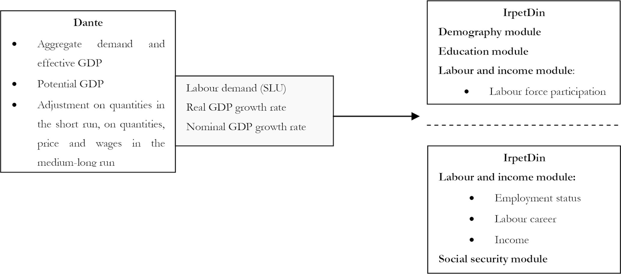
IrpetDin models employment decisions partly differently. First, it simulates labour supply. Then, it takes labour demand from the IRPET’s structural econometric macro model called “Dante”. Finally, it matches exogenous labour demand with endogenous labour supply (Figure 3). The two models are not integrated; IrpetDin simply aligns labour demand and GDP growth rates to Dante’s estimations. The purpose of the alignement to Dante is to make coherent IRPET’s microsimulation model and macro model.

IrpetDin’s alignements to Dante.
The following paragraphs provide details of the labour and income module.
7.1. Labour supply
In each year of the simulation period, immediately after the education module, labour supply is composed of employed ( ) and unemployed individuals ( ) from the previous year. However, inactive people from the previous year and students who completed their education in year could become active and start to participate in the labour market.
We calculate participation rates, by age, by gender, by level of education, by role within the family (head of the family or not) and by territory (Italy or Tuscany), based on ISTAT’s Italian Labour Force Survey. We then activate inactive people from the previous year, if their inactivity has been lower than 3 years for women8 , as well as students who finished school or university in year , whether they obtained a diploma/degree or dropped out. If the random number is lower than the probability, then the candidate becomes active and enters the labour market as a job seeker. Labour supply in each year t (S t ) is therefore composed of the sum of employed at ( ), unemployed individuals at, t – 1, ( ), and the new flow of job seekers ( ) (1). The sum of and is the total number of unemployed individuals in each year t, ut .
7.2. The macro model and labour demand
Dante is a structural econometric macro model, developed by IRPET, which analyses economic structural changes and the effects of policies in Italy. Since it is designed to evaluate regional policy, Dante distinguishes between three Italian macro-regions: Centre-North, South and Tuscany, all of which are linked together using an interregional trade matrix9.
It is based on post-Keynesian theories and may be classed as a stock-flow consistent model. The complete structure of the model contains a rather complex set of behavioural equations and accounting identities. The following are some essential features of the model.
Goods and services market. Aggregate demand is a function of private and public consumption, investments and exports. The relationship between output and factors of production is based on a Leontief production function. Factors of production are therefore used in fixed proportions, since there is no substitutability between factors in the short run10. Potential output is determined by the maximum rate of use of labour and capital11. Actual output is equal to the level of aggregate demand.
Labour market. Labour supply is exogenously aligned to the participation rates predicted by ISTAT. Labour demand, expressed in standard labour units (SLU)12 , is given by the ratio between actual output and labour productivity13. SLUs are converted into the number of workers through a coefficient that measures the average ratio between SLUs and numbers of workers. Labour demand, expressed in number of workers, is then compared with labour supply in order to predict unemployment or job vacancies.
Adjustment mechanisms. Unlike neo-classical models, in the short run, excess/insufficient aggregate demand compared with potential output is only adjusted through quantities and not through wages and prices. Therefore, if aggregate demand is lower than potential output, then labour demand is lower than labour supply and the model predicts an increase in unemployment. In the medium-long run, adjustments may also be made through wages and prices. If aggregate demand exceeds potential output, because, for example, there is a labour supply shortage, then wages and labour costs increase and companies in turn increase the prices of goods and services, with potentially depressing effects on aggregate demand, actual output, labour demand and employment.
Dante is able to analyse economic structural changes up until 2035. IrpetDin therefore takes labour demand data from Dante, expressed in SLU and broken down by sector of activity (public or private), until 203514. For the following years, IrpetDin assumes a growth rate in SLU equal to the average of the previous few years.
7.3. Matching between labour demand and supply
Labour demand data from Dante does not include workers receiving redundancy funds (RF). IrpetDin therefore uses administrative data from INPS, Italy’s National Social Security Institute, regarding the number of hours of redundancy funds in order to estimate the number of workers involved with the social safety net and to simulate scenarios about their evolution over time. More specifically, we estimate SLUs receiving RF by dividing the number of hours by an average standard working time. We then add the SLUs receiving RF to the labour demand, expressed in SLU, derived from Dante.
Dante makes projections about labour demand by sector of activity. IrpetDin breaks down labour demand within the various sectors by level of education, applying the proportions observed in terms of companies’ intention to hire staff, as expressed in the Excelsior survey15. However, IrpetDin allows us to hypothesise different scenarios regarding the proportions of labour demand by sector and level of education over time.
In the basic scenario, IrpetDin converts the labour demand originally expressed in SLU into workers, using the same ratio between SLUs and number of workers used in Dante. However, the model also allows us to conjecture a different evolution of the ratio in the future, depending on assumptions about working time.
Given the peculiar characteristics of the Italian labour market, IrpetDin models the matching of labour demand and supply by sector, by level of education and by nationality. Indeed, a distinctive feature of the Italian labour market is its mismatch of particularly highly skilled individuals. According to Adda et al. (2017) the incidence of over-skilling is especially high among graduates (20%) and individuals with secondary education (14%). Another distinctive feature concerns the type of migration. Unlike continental Europe or northern countries, migration in Italy is a relatively recent phenomenon and migrants are generally lower skilled. As described by the Ministero del Lavoro e delle Politiche Sociali (2019), the employment rate is higher for migrants than native Italians and migrants are typically employed in low-skilled job positions.
IrpetDin models the matching between labour demand and supply by taking these distinctive features of the Italian labour market into account. Given the high level of over-skilled graduates in Italy, we assume that unsatisfied graduates, who do not find a job requiring tertiary education, go on to compete for jobs requiring secondary or even only primary education. Furthermore, we assume that individuals with secondary education, who do not find a job requiring secondary education, go on to compete for jobs requiring just primary education. We then hypothesise a sort of priority among migrants for jobs requiring primary education.
More specifically, the matching is completed in the following way, for each time frame and sector of activity . With regard to labour supply, we initially only consider individuals who are already employed at time . If labour demand, , is lower than the number of those employed at the time , , then the sector has an over-supply (2). Consequently, we fire workers according to the ratio between over-supply and labour demand .
If labour demand, , is higher than the number of those employed at the time , , then the sector has an over-demand (3). We then hire individuals among the remaining part of labour supply, composed of unemployed individuals to the following rules.
We start from jobs requiring tertiary education (4). If labour demand for tertiary education is higher than the number of unemployed graduates , then everyone finds a job with a probability equal to 1, otherwise they find a job with a probability equal to . Unsatisfied graduates compete with individuals with secondary education for jobs requiring secondary education, again with a probability equal to 1 if labour demand for secondary education is higher than the sum of labour supply with secondary education and unsatisfied graduates, or equal to the ratio if labour demand is lower (5).
IrpetDin then continues with jobs requiring primary education. Initially, only foreign workers compete for low-skilled positions. If labour demand is higher than foreign labour supply, then every foreigner can find a job with a probability equal to 1 and low-skilled Italian workers compete for the remaining positions after foreigners have been hired ( ) (6). If labour demand is lower than foreign labour supply, then only foreigner workers can find a job with a probability of (7).
The procedure that we use for the matching simulates labour market transitions-from unemployment to employment and vice versa-only when an imbalance between labour supply and demand by sector occurs. Our partial omission of churning can be a strong drawback, especially in view of the increase in temporary work that happened in the last two decades and will probably continue in the future. IrpetDin could, therefore, over-estimate stable careers, accumulation of social contributions, pension requirements and amounts.
Further, our matching between labour demand and supply does not provide any long run price/wage adjustments. We are, therefore, implicitly assuming that no kind of adjustment of the imbalances can take place except in the quantities.
Another important shortcoming is our implicit assumption of the absence of employment/unemployment lasting less than one year. This is a significant limit when we use IrpetDin to evaluate the effects of pension reforms, such as those implemented in 2019, that change pension requirements even for fractions of a year.
After hiring and firing individuals, IrpetDin predicts the unemployment rate16. Thanks to the modelling of labour dynamics by level of education and by sector, IrpetDin can also predict a sort of qualitative mismatch, whereby individuals are hired for jobs requiring a lower level of education than they have.
7.4. Career and incomes
After attributing employment status, IrpetDin simulates types of work, careers and working time. We divide workers into self-employed individuals and employees by applying the proportion observed in the current stock of workers. We then simulate career progressions for employees, from blue-collar worker to white-collar worker, to manager and then from manager to executive, by sector of activity. Transition rates are calculated based on the Italian Labour Force Survey and are then attributed to employees. Part-time work is imputed after estimating a model for the probability of being employed part-time depending on gender, age and number of children. In order to stabilize the value we estimate the probability of being employed part-time on five waves of the Italian Labour Force survey (2009-2013). Given that in Italy part time work has been strongly affected by the economic crisis of 200917 we estimate a second model, with the same covariates, on the two waves 2018 and 2019 of the Italian Labour Force survey. Table A4, attached hereto, shows the estimation results of the two models. We use pre-crisis probabilities until 2017 and post-crisis ones from 2018. As we will described in paragraph 10, we assume a return to pre-crisis probabilities in the long run from 2030 onwards.
The final step of the labour and income module is to attribute incomes to individuals who are already employed and new recruits. We estimate a standard Mincer equation for the logarithm of income depending on workers’ characteristics (territory, age, gender, contributory seniority, level of education, employment status, number of hours worked, citizenship), separately for self-employed individuals and employees, based on EU-SILC 2008 data (please see tables A5 and A6, attached hereto, for the estimation results). The estimated coefficients and the distribution of the error term are used to impute incomes18. For individuals who are already employed, yearly income is calculated by applying estimated coefficients to their changing characteristics (such as age, seniority, qualification, working time) and fixed characteristics (gender), and by adding the difference between their true and estimated yearly income in 2008. For new recruits, income is calculated by applying estimated coefficients to their characteristics and adding an error term, randomly extracted from the distribution of error terms estimated by EU-SILC for workers in 2008.
IrpetDin assumes that incomes grow over time in line with the nominal GDP growth rate, taken from Dante.
8. Social security module
The social security model is mainly characterised by deterministic events, such as pensions and social assistance for the elderly. The implicit subsidy given by the public provision of health services is imputed to each individual depending on their characteristics. A probabilistic procedure, on the other hand, is only used for individuals who are not self-sufficient. Other social security transfers, which have less of a financial impact, are not simulated in the model, such as unemployment benefits, transfers to families with children and minimum income to prevent poverty.
8.1. Old-age and seniority pensions
In Italy, the pension system has been reformed many times in order to make it financially sustainable and fair between generations. Typically, implementation of these reforms is postponed or revised, in order to make them more acceptable to current generations, which actually ends up offloading costs onto future generations.
The most important reform, the so-called Dini Reform in 1992, had precisely these characteristics. The reform, which shifted from Defined Benefit (DB) pensions to Notional Defined Contribution plans (NDC), was not applied to individuals who were retiring in those years, but rather to those who entered the labour market after 1995.
Specifically, the Dini Reform introduced three different regimes: i) the DB plan for workers with more than 18 years of contributions in 1995; ii) the NDC plan for workers who started working after 1995; and, iii) a mixed plan for workers with contributions of between 1 and 18 years in 1995. The method used to calculate the pension amount differs for the three regimes. For retirees with the DB regime, a full DB plan is applied; for retirees with the NDC regime, a full NDC is applied; for those with the mixed system, a DB plan is applied for the years before 1995 and an NDC plan is applied for the years after 1995 (the so called “pro-rata”).
The Dini Reform was followed by other reforms, whose objectives were, respectively, to increase pension eligibility requirements, to solve financial sustainability problems, or to correct the previous reforms, mainly for electoral issues. In 2011, an important reform was introduced (Italian Law no. 214/2011, the so-called “Fornero Reform”) with the aim of making the system more financially sustainable and fair between generations. The Fornero Reform increased the retirement age, linked retirement requirements automatically to increases in life expectancy and partially extended the NDC plan to all people retiring, also for workers with more than 18 years of contributions in 1995, for years after 2012. Therefore, following this reform, there are two regimes, the mixed and the NDC regime. The two regimes are applied both for old-age pensions and seniority pensions.
IrpetDin simulates the current pension rules, which were once again changed in 2019 with the so-called “quota 100” reform (Italian Law no. 26/2011)19. It starts by identifying and attributing the pension regime, either mixed or NDC, for each worker in the sample and then calculates the pension amount for both regimes.
The calculation rule for the DB plan can be represented as in (8). The pension amount is determined by multiplying the average income of the last 10 years for employees and 15 years for self-employed workers20 ( ) by a rate of return ( and by the number of working years ( ). The rate of return decreases with income classes21.
The calculation rule for the NDC plan can be represented as in (9). The pension amount is determined by multiplying the total amount of social contributions paid during working life, capitalised at the rate of GDP growth ( ) by a transformation rate ( ). The transformation rate is a value that transforms the amount of contributions into annual pension income; it increases with retirement age and increases over time.
After calculating the pension amount, IrpetDin simulates pension eligibility requirements for old-age pensions and seniority pensions, as established by the law. Requirements increase over time as life expectancy increases, although in 2019 the so-called “quota 100” reform blocked any increases to the retirement age until 2026. The simulation of requirements comes after the calculation of the pension amount because Italian law provides workers in the NDC regimes and those receiving old-age pensions with a form of flexibility to retire before the retirement age, if their pension amount is higher than certain thresholds.
By default, IrpetDin simulates retirement for anyone who meets pension eligibility requirements. However, for old-age pensions, it allows us to simulate the choice of whether to retire or not. Specifically, the model calculates the replacement rate, i.e. the ratio between the pension amount and the last working income. If the replacement rate is higher than a certain level, decided by assumption, then the workers retire, otherwise they continue to work.
Finally, IrpetDin simulates survivor pensions for those whose spouse has died and indirect pensions for children whose parents have died.
8.2. Social assistance and minimum pensions
Italian social security provides some forms of social assistance for the elderly and retirees. IrpetDin simulates the eligibility requirements and the amounts established by Italian law.
There is a minimum pension supplement, representing an integration of the pension amount up until a specific minimum income threshold, for retirees who live in households22 with an income below certain levels (in Italian, the so-called “integrazione al trattamento minimo”). An additional supplement (in Italian, the so-called “maggiorazione sociale” ) is provided to retirees over the age of 70, depending on their household income.
Finally, for those aged 65 and over, the Italian welfare system provides a form of non-contributory social assistance, financed through general taxation, known as the “assegno sociale”. This is a sort of minimum income to prevent poverty, subject to means testing and proven with a top-up mechanism, which, however, is only for the elderly.
8.3. Health in-kind transfer
IrpetDin includes a simplified simulation of the implicit subsidy that people receive from public health services (so-called “in-kind” transfers). In-kind health transfers are only attributed to people living in Tuscany, in relation to which we have detailed regional administrative data.
Two different approaches to including in-kind transfers in microsimulation models can be found in the literature: the actual consumption approach and the insurance value approach. The actual consumption approach only imputes the monetary value of in-kind transfers to individuals who actually use the service. The insurance value approach imputes an average monetary value of in-kind transfers to every individual, based on demographic characteristics (usually age and gender), without taking into account the actual use of services.
We apply the insurance value approach, widely used in literature for health services, for hospital, specialist and pharmaceutical services. We calculate average per-capita expenditure by gender, by age, by level of education and by nationality for hospital services; by gender, by age and by nationality for specialist services; and by gender and by age for pharmaceutical services.
8.4. Disability and long-term care
The last social security transfer simulated in IrpetDin is long-term care (LTC) for people who are not self-sufficient. As LTC is a strictly age-related benefit, the evolution of the number of people who are not self-sufficient could be very significant for national and regional policymakers.
We estimate the probability of being disabled based on an ISTAT survey, broken down by age, by gender and by level of education (please see table A7, attached hereto, for the estimation results) and, accordingly, we impute disability and non-self-sufficiency to all people in the sample. Public expenditure for LTC is estimated based on official data from the Italian Ministry of Finance and is then attributed to disabled people.
9. Validation
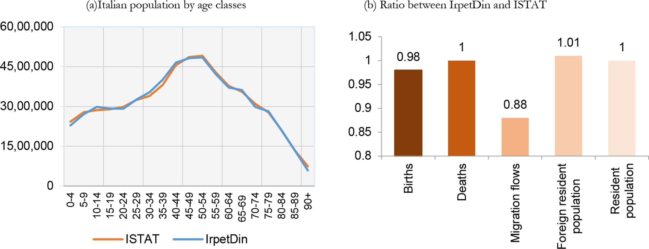
As mentioned previously, before using IrpetDin, we validate our simulations until actual data is available. Figure 4a compares IrpetDin’s simulation of the distribution of the Italian population by age classes in 2017 with official ISTAT data, with clearly satisfying results. Figure 4b compares some 2017 stock and flow indicators from IrpetDin with the equivalent ones registered by ISTAT. As the ratio clearly shows, there are only small differences, with a tendency to only underestimate migration flows.

Validation of demography. Year 2017. Italy.
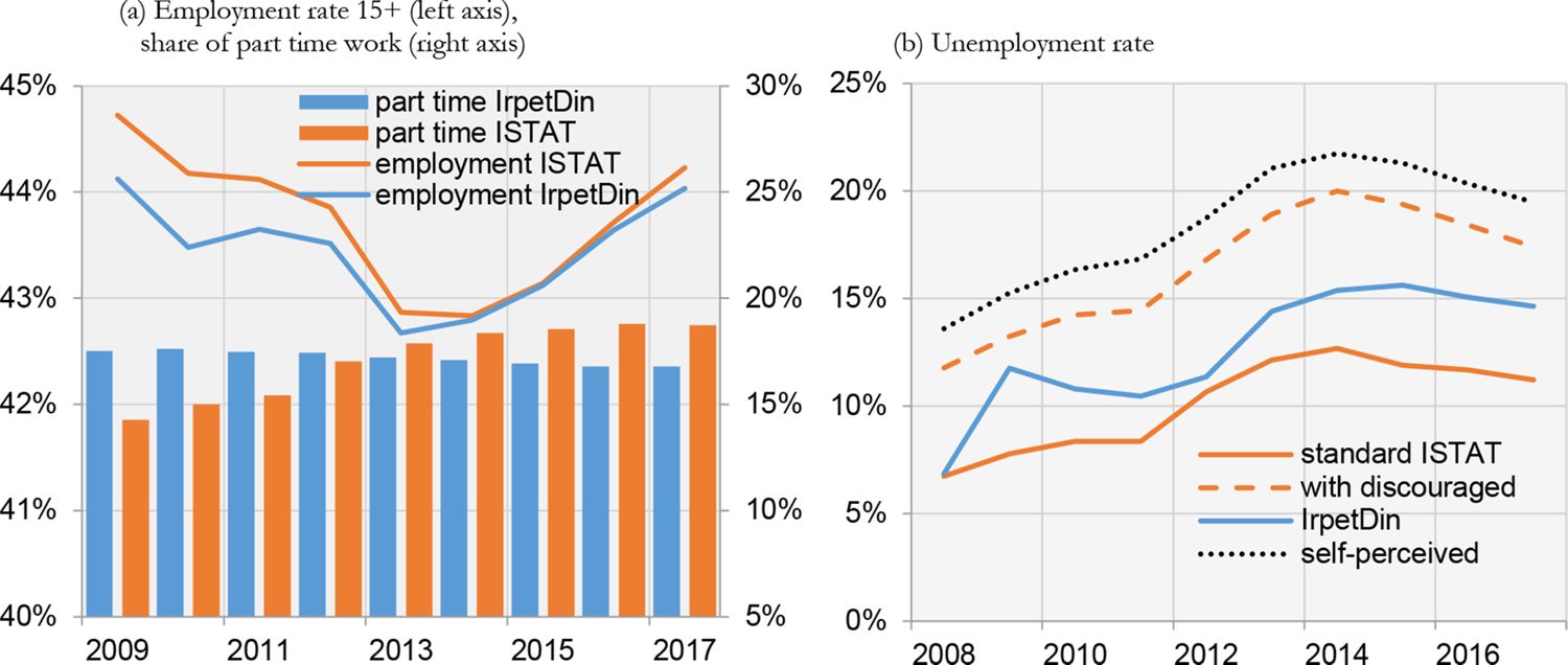
The simulated employment rate is close to the actual rate (Figure 5a-left axis). The model tends to overestimate part time work until 2012 and to underestimate from 2013 (Figure 5a-right axis). However, considering the average of the entire period the share of part time work is around 17,1% in both the simulated and the actual data.
The simulated unemployment rate is overestimated (Figure 5b). However, IrpetDin does not identify unemployed by applying the official definition used by ISTAT to measure unemployment rate, according to which unemployed are people of working age actively seeking work and available to start working before the end of the two weeks following the reference week of the survey. Indeed, IrpetDin’s unemployment rate is somewhere in between the official rate and the rate that includes among unemployed also people jobless who do not actively seeks for a work (discouraged people) or the rate of those self-declaring unemployed (the so called “subjective” definition of unemployment) (Figure 5b).
Validation of labour market indicators. Italy.
With regard to pensions, IrpetDin achieves satisfactory results in terms of stock and flows of retirees and in terms of pension expenditure with respect to official data (Table 1).
Validation of pensions. Italy
| IrpetDin | ISTAT | Ratio IreptDin ISTAT | |
|---|---|---|---|
| Stock of retirees in 2017 | 10,800,000 | 11,039,137 | 0.98 |
| Pension flows 2016-2017-2018 | 284,138 | 291,115 | 0.98 |
| Pension expenditure (billion euro) in 2017 | 236 | 232 | 1.01 |
-
Source: IrpetDin, ISTAT.
10. Main simulation results
Having validated the model, we can now take a look at IrpetDin’s predictions for the future. Results are based on assumptions about the exogenous indicators/variables reported in Table 2. In the basic scenario, life expectancy, fertility and migration flows are all aligned with ISTAT’s central forecast for the 2017-2065 period. Real and nominal GDP growth rates are in line with Dante up until 2035, after which they are based on our assumptions. Labour demand is taken from the basic scenario of the Dante macro model. The SLU/employed ratio is assumed to decrease by -0.2% until 2020, after which time it remains unchanged. The labour income growth rate is the same as the nominal GDP growth rate. We assume a part time work share in line to the post-crisis level (2018-2019) from 2018 until 2030 and a return to pre-crisis level from 2030 onwards. Social security is simulated by following current legislation without any changes in the future, except those provided for by the law.
We simulate a second scenario, that we called “official”, in which we change some assumptions on the economic trends with respect to the basic scenario. Specifically, we assume the SLU/employed ratio underlying the assumptions on employment and unemployment of the last official report of the Italian Ministry of Finance on the evolution of pension expenditure in the long term (Ragioneria generale dello Stato, 2020). Further, we increase the number of years of inactivity after which women definitely leave the labour market (from three to eight from 2025) in order to align our labour supply to the one assumed in the official report of the Italian Ministry of Finance. Compared to our basic scenario, the official scenario predicts lower unemployment in the short term and higher in the long term. In the following, we describe the simulation results under the basic scenario and we compare the distributive effects on retirees between the basic scenario and the official one.
Exogenous indicators/variables
| Indicator/variabile | External source | |
|---|---|---|
| Demographic trends | Life expectancy | ISTAT forecast, central scenario |
| Fertility | ISTAT forecast, central scenario | |
| Migration flows | ISTAT forecast, central scenario | |
| Economic trends | GDP real growth rate | Dante until 2035, then our assumption |
| GDP nominal growth rate | Dante until 2035, then our assumption | |
| Standard Labour Units | Dante until 2035, then our assumption | |
| Ratio SLU/employed | Our assumption | |
| Labour income growth rate | Our assumption | |
| Part time work | Our assumption | |
| Social security programmes | Pensions and social assistance for old-people | As current legislation |
| Health and long term care | As current legislation | |
| Health and LTC costs growth rate | Our assumption |
10.1. Simulation results under the basic scenario
According to IrpetDin, the demographic dependency, measured by the ratio between the number of over 65s and those aged between 15 and 64, will increase from 35% in 2018 to 60% in 2050 (Figure 6a). Demographic dependency figures for Tuscany are even worse, where the ratio will increase from 40% in 2018 to 74% in 2050 (Figure 6b).
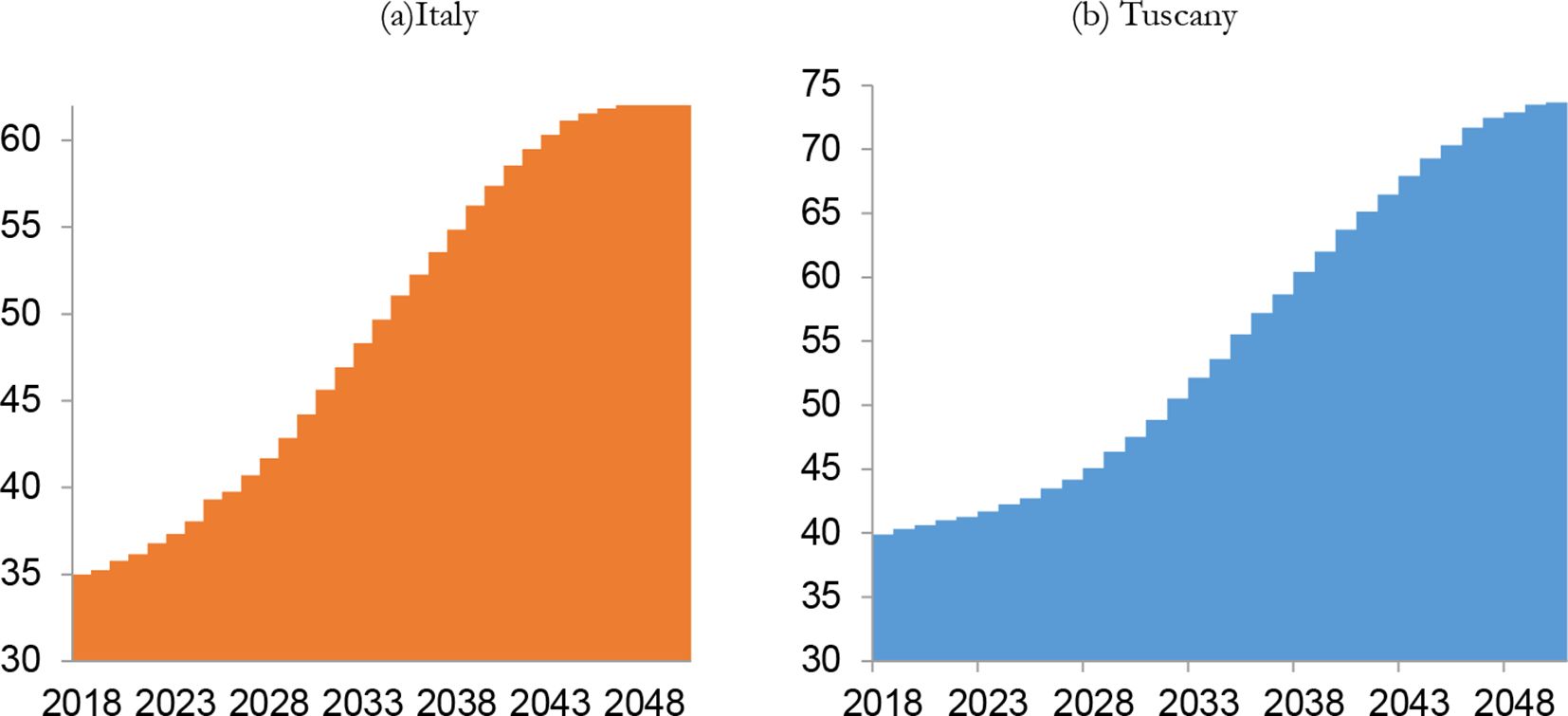

Demographic dependence for Italy and Tuscany (%).
The percentage of individuals aged between 18 and 34 with tertiary education will increase in the future, but this will not be enough to reach the level of other European countries, at least not in the next 30 years (Figure 7a). The percentage of people who only have primary education will decrease up until 2030, after which it will become stable at about 15% (Figure 7b).
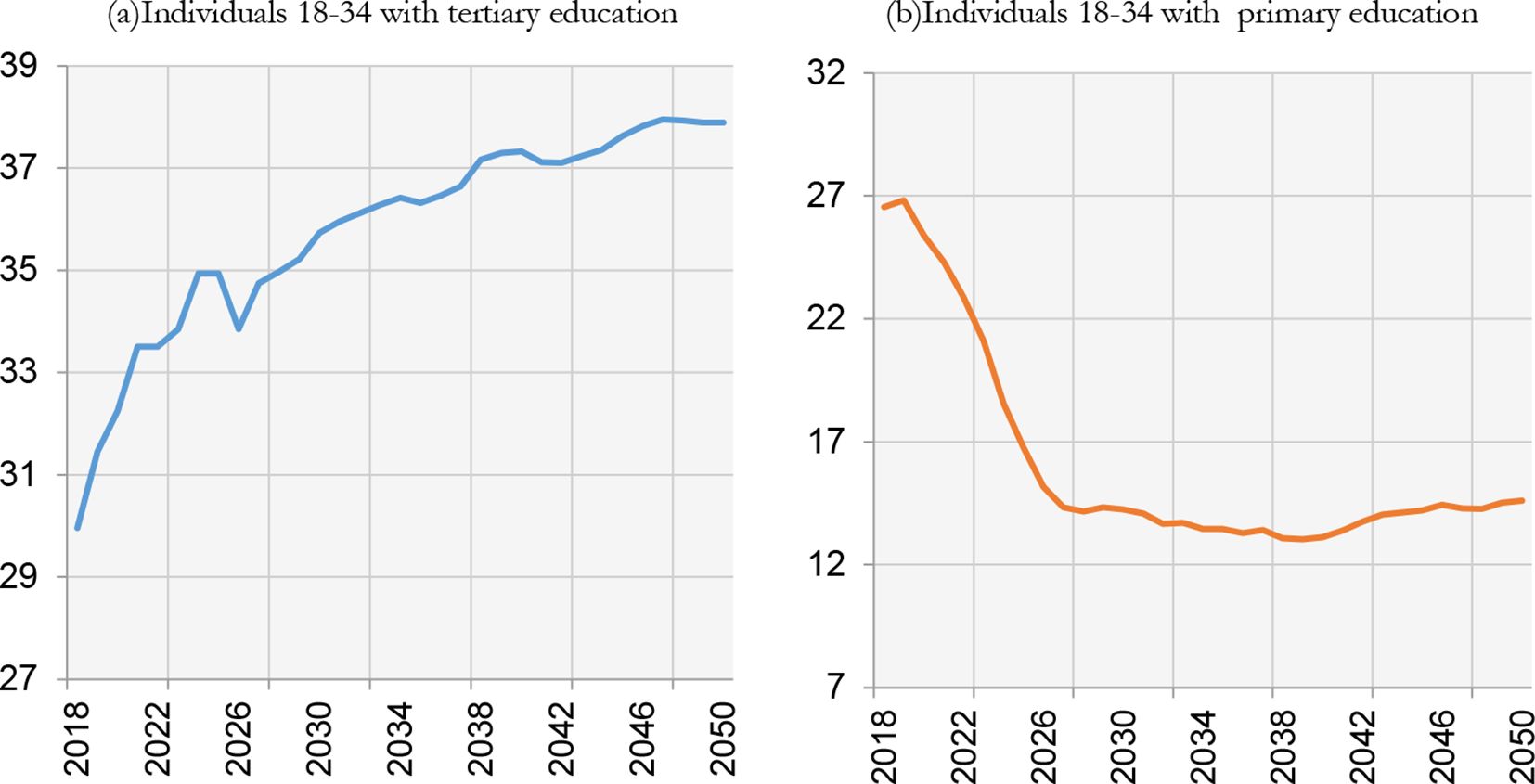
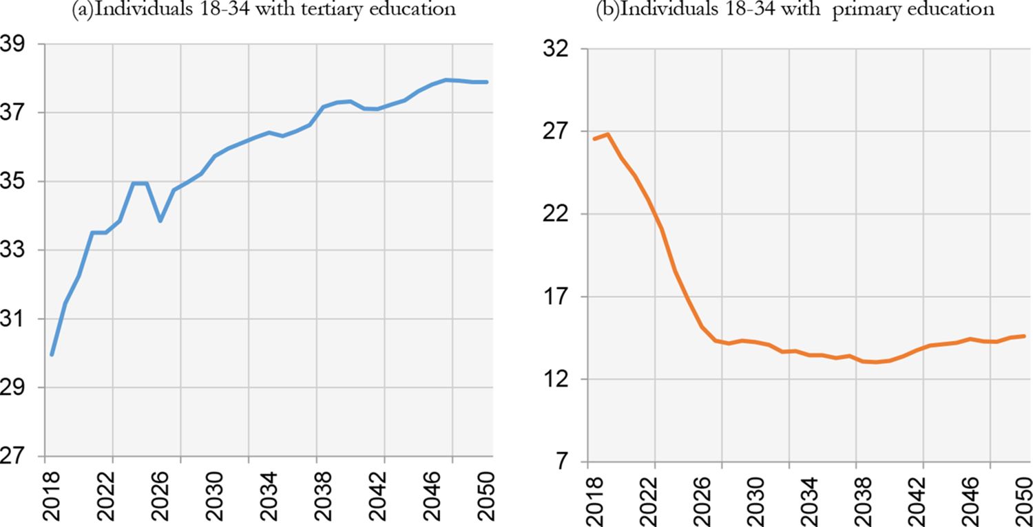
Education. Italy.
With regard to the labour market, the model predicts a strong decrease in labour supply (Figure 8a). In the first years of the projection period, the workforce aged between 35 and 55 decreases due to the fall in the birth rate. Elderly workers, on the other hand, do not diminish as they continue to work due to pension reforms. Starting from 2044, the drop in younger workers is no longer offset by the growth in the number of older workers. The numerous baby boomers will begin to retire and leave the labour market (after the postponement introduced by Italian Law no. 214/2011). Similar results are described for an other microsimulation model (Caretta et al., 2012). Indeed, they predict a sharp increase in employment rates for old workers (especially female) for the next 20 years until a stabilisation in around 2040.
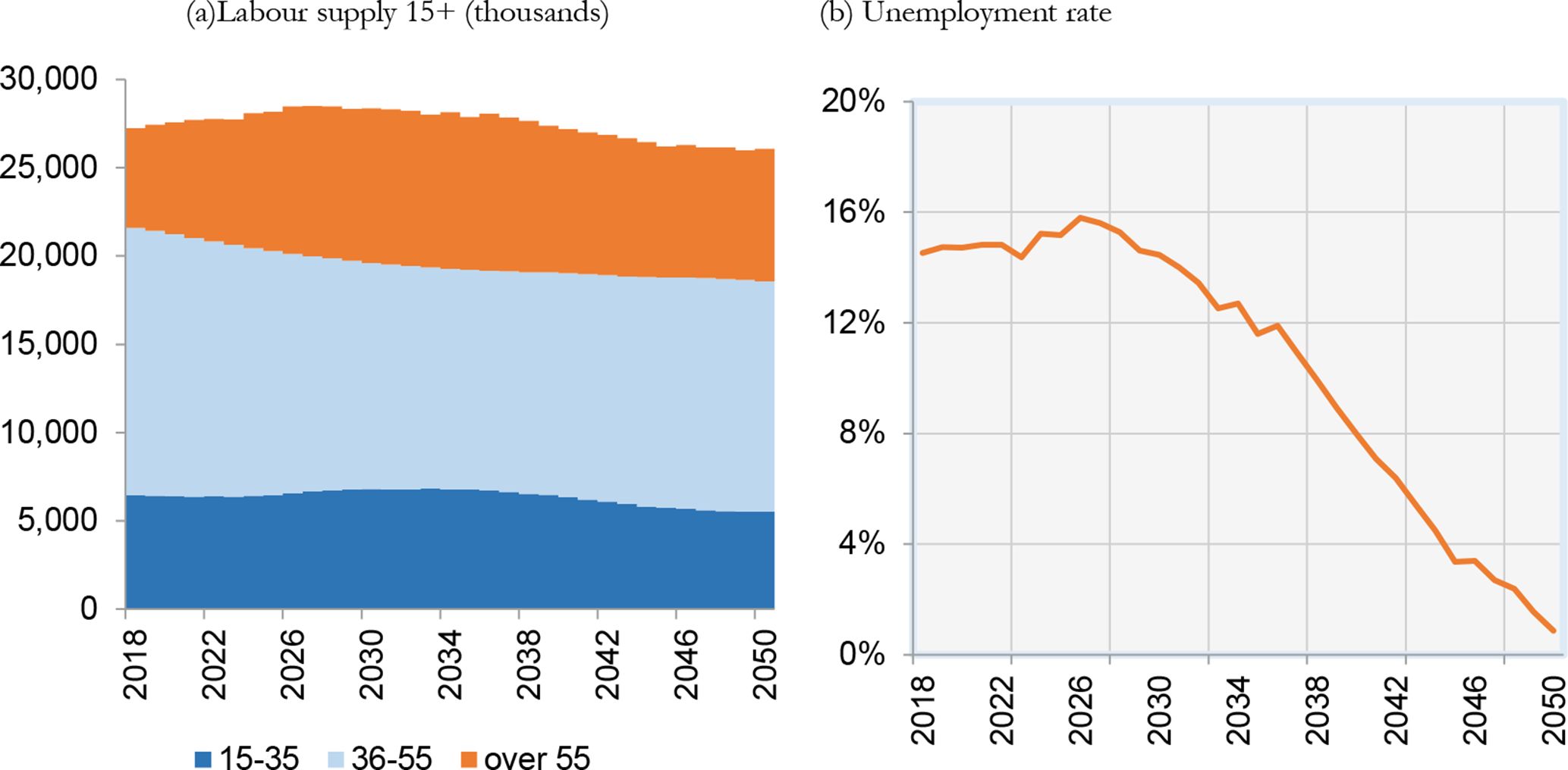

Labour supply and unemployment. Italy.
Consequently to these dynamics, IrpetDin predicts a diminishing labour force in the long run. With demand growing by around 2.5 million units during the period, according to our projections and in line with the Dante macro model, the unemployment rate will converge to a value that we may define as structural in 2040 (Figure 8b). It then reduces to zero.
Given the growth in labour demand and the diminishing labour supply, the model predicts a gradually decreasing quantitative mismatch, i.e. the difference between labour demand and supply (Figure 9a). According to IrpetDin, the qualitative mismatch will decrease until 2038 (Figure 9b). As in the baseline scenario, the proportions of labour demand by level of education will not change over time, with the reduction in the qualitative mismatch strictly depending on the shortage of labour supply with respect to labour demand.
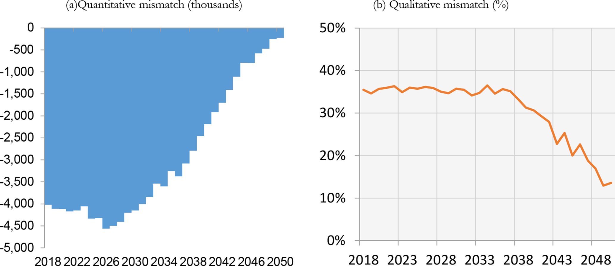

Quantitative and qualitative mismatch. Italy.
There is a high rate of people retiring between 2025 and 2044 due to the baby boom generations retiring (Figure 10a). We will have flows of retirees with the old DB plan (which became mixed after the introduction of Italian Law no. 214/2011) and the mixed plan, until 2039. The stock of retirees will increase until 2045 and will then become stable (Figure 10b).
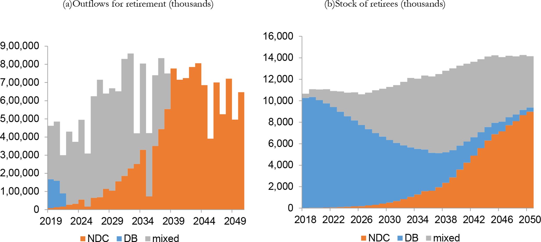

Pensions flows and stocks. Italy.
Replacement rates will strongly decline in the future, especially for self employed workers (Figure 11a). In the long run, we will therefore face a problem of intra-generational equity, with retirees with very low pensions. On the other hand, the Gini among retirees will decrease, as differences among retires shall diminish when the NDC plan fully comes into force (Figure 11b). A decreasing in the Gini among Italian retirees in the very long run was also found in Caretta et al. (2012).
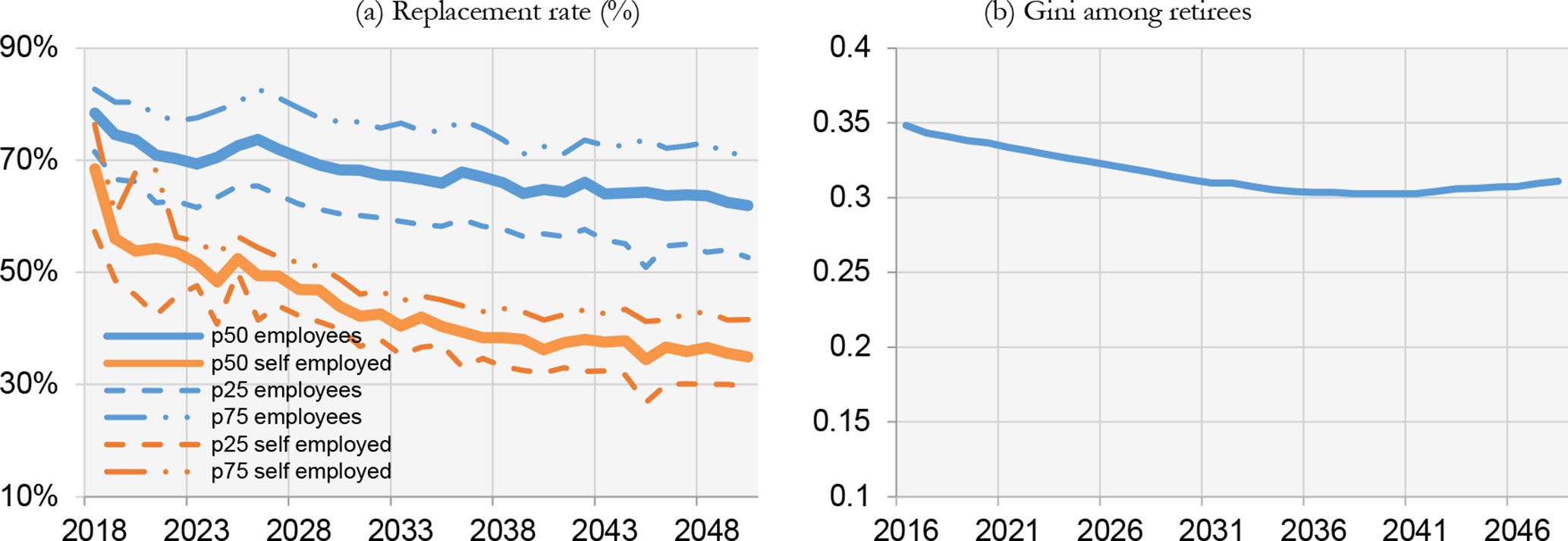

Pensions: intra-generational equity. Italy.
The pension expenditure to GDP ratio will decrease from 2045, when the number of retirees will become stable (Figure 12a). In order to evaluate inter-generational sustainability we use the ratio between the future pension amounts and the accumulated contributions amounts for the flow of retirees (the so called “net present value ratio”). If the ratio is over 1 the pension system is not fair between generations. As can be easily seen from Figure 12b, the NDC plan will make the Italian pension system more fair between generations only in the very long run.
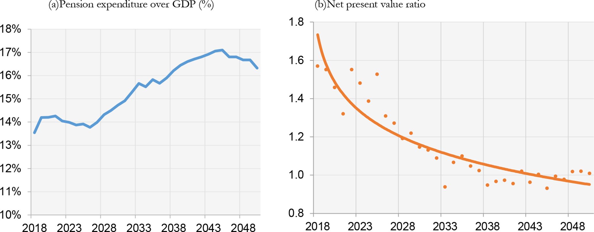

Pensions: financial sustainability and inter-generational equity. Italy.
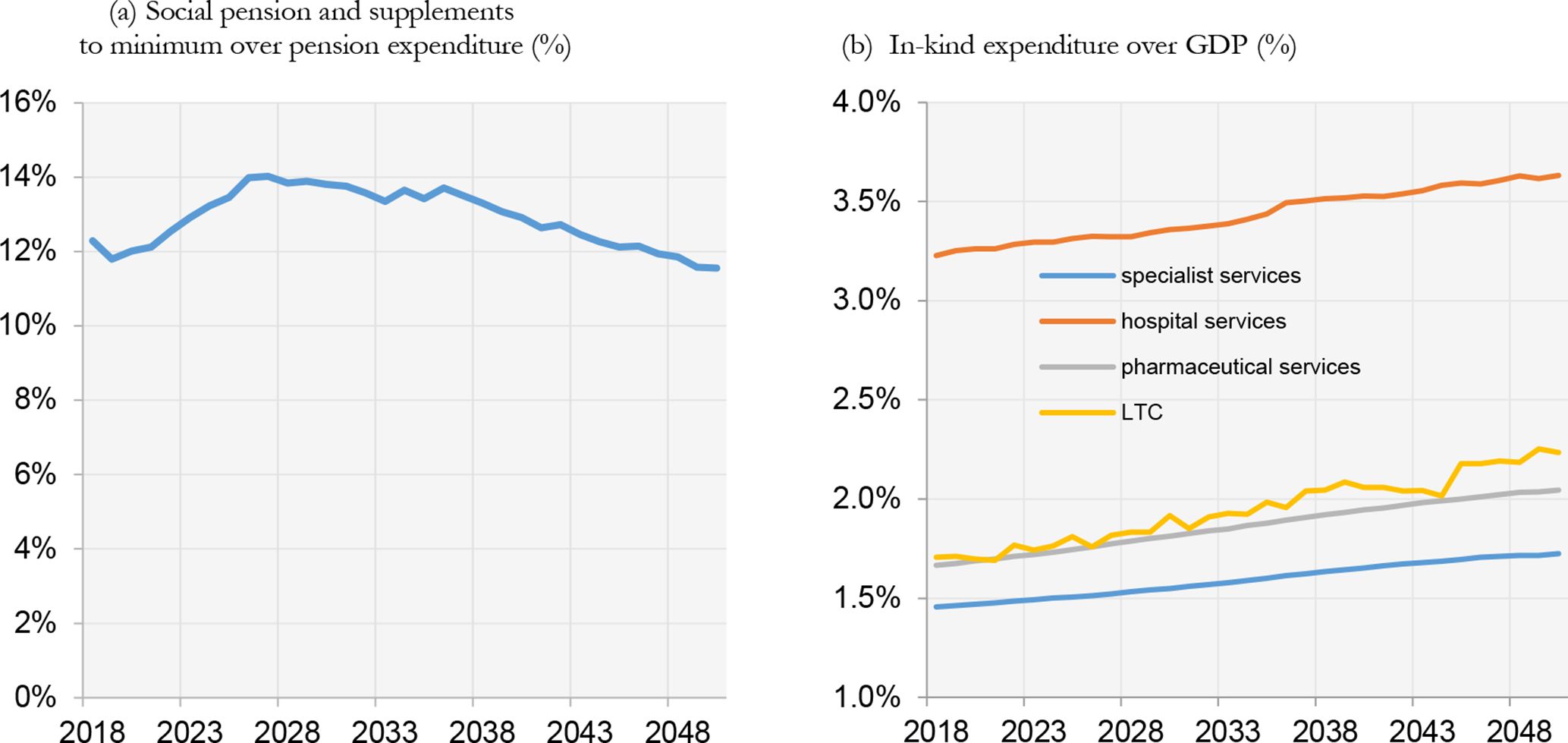
As in Marano et al. (2012), the Italian expenditure for social assistance for old people, composed by social pensions and supplements to minimum, will increase in the future (Figure 13b). However, IrpetDin predicts a decrease starting from around 2040, when supplements to minimum will not be in force anymore (Figure 13a).

Social assistance for old people and in-kind services.
Finally, IrpetDin predicts a linear but not sharp increase in expenditure for in-kind transfer, composed by specialist, hospital, pharmaceutical services and long term care (Figure 13b).
10.2. A comparison of distributive effects between the basic and the official scenario
In this paragraph we compare the distributive effects on retirees between the basic and the official scenario. As explained in the previous paragraph, the official scenario differs with respect to the basic one in the assumptions on economics trends. As can be seen from Table 3, in the official scenario the unemployment rate is lower until 2032 and higher from 2033 onwords than the basic one. In order to evaluate the distributive effect on retirees of this change we measure the 25th and the 75th percentile of the of replacement rates for employees and employed and the Gini coefficient on retirees (see Table 3).
Unemployment rate, percentiles of replacement rates for employees and employed, Gini among retirees
| 2018-2032 | 2033-2042 | 2043-2050 | ||
|---|---|---|---|---|
| Basic scenario | Unemployment | 11,3% | 4,6% | 0,1% |
| p25 employees | 62,4% | 57,8% | 54,0% | |
| p75 employees | 78,5% | 74,2% | 72,4% | |
| p25 self-employed | 42,5% | 34,0% | 30,1% | |
| p75 self-employed | 53,4% | 43,7% | 42,2% | |
| Gini | 0,322 | 0,305 | 0,305 | |
| Official scenario | Unemployment | 9,7% | 6,8% | 5,4% |
| p25 employees | 62,4% | 58,0% | 54,2% | |
| p75 employees | 78,5% | 74,3% | 72,5% | |
| p25 self-employed | 42,5% | 34,1% | 30,2% | |
| p75 self-employed | 53,4% | 43,8% | 42,2% | |
| Gini | 0,322 | 0,305 | 0,305 |
Not surprisingly, in the first period, 2018-2032, there are not differences in replacement rates. The impact on pensions can occur at least with a certain temporal lag with respect to labour market changes. Those that occur during the last ten years, 2040-2050, will have effects only after our observation period (beyond 2050).
Indeed, some differences emerge only after 2033 and specifically the model predicts a mild increase in replacement rates, both at the top and the bottom of pensions distribution, under the official scenario. This effect depends on the lower unemployment rate in the short run (2018-2032) assumed in the official scenario compared to the basic one, that increases earnings and pension contributions and, consequently, the pension amount. Probably, given that replacements rates increase both at the top and the bottom of the distribution, we do not observe any impact on the Gini index.
Conversely, we can not observe in our observation period, ending in 2050, the effects on pensions of the higher unemployment rate assumed in the official scenario compared to the basic one for the medium and, most of all, for the long run (2043-2050).
11. Conclusions
Firstly, especially since it is modelled in great detail, IrpetDin takes a very long time to execute the entire period 2008-2050. A translation of the SAS code in a programming language, like C++ or Java, could improve the speed of execution.
Secondly, even if IrpetDin aims at best predicting labour market indicators some validation problems in replicating official unemployment rates still remain. Further future research is therefore necessary regarding this issue.
Thirdly, some information imputed in IrpetDin, like historical working experience, may be available trough to an integration between EU-SILC and administrative data, as made in other Italian microsimulation models. In the future, it is desirable to follow this approach in IrpetDin too.
Last but not least, IrpetDin simply aligns labour demand to an external macro model. A further development could be the integration between IrpetDin and IRPET’s macro model, through a joint micro-macro model.
Footnotes
1.
We removed a part of observations who are 0 years old, otherwise the adjustmet to real data was not feasible.
2.
The individual with the minimum sample weight is consequently not repeated.
3.
According to official data by ISTAT, even if the age at which people get married is increasing, the percentage of those with more than 60 years old are residual, expecially among women.
4.
We have overall 729 rates for each territory.
5.
According to official data by ISTAT, the percentage of divorces before three years of marriage is not residual (about 10% of total dissolutions), but we chose this threshold for possibile issues of sample representativeness.
6.
According to the survey, the majority of single individuals leaves home within 50 years old.
7.
Mobility between sectors and qualifications are usually not modelled.
8.
According to Cataldo and Tosi (2012), women may be discouraged from participating in the labour market because of the lack of adequate educational services for children and depending on their working experience. They estimate an higher probability to become inactive in a given year if a woman was unemployed or employed with non-standard contracts in the previous year. Pacelli et al. (2012) demonstrate that the probability of exiting from employment depends on age, having children, income, firm size. In our model we assume the ultimately exit from the labour after 3 years of inactivity.
9.
Dante considers 30 industries and 59 commodities.
10.
In the long run proportions can change for several reasons, among which technological progress.
11.
It takes into account also the average unemployment rate of the last few years.
12.
Standard labour units measure the number of job positions that correspond to standard workers, i.e. full time workers.
13.
Productivity is endogenously determined within the model.
14.
IrpetDin also takes from Dante real and nominal GDP growth rates.
15.
Unioncamere – Minister of Labour, Excelsior survey.
16.
A comparison of the predicted unemployment rate with the one estimated by Dante gives similar results. In some past experiences we linked IrpetDin and Dante with iterations. Dante computed labour demand as input for IrpetDin. IrpetDin predicted participation rates as input for Dante. Dante computed again labour demand as input for IrpetDin, an so on, until unemployment rates predicted by Dante and IrpetDin converge.
17.
As clearly stated by Istat, Ministero del Lavoro, Inps, Anpal, Inail (2019) part time work strongly increased after the great recession of 2009 , owing to involuntary part time, used by firms as a strategy to tackle the economic recession. Precisely, part time increased starting from 2011 until it stabilizes from 2018. As a result, in 2018, the share of part time work in Italy is more in line to the european average (18,6% vs 20,1%) but involuntary part time is some three times higher (64,1% vs 23,4%).
18.
For simplicity in our Mincer equation we do not correct for selection bias. Consequently, we could over-estimate the returns to education.
19.
This last reform made less stringent pension eligibility requirements.
20.
For working years before 1992 the average of the last 5 and 10 years is respectively considered for employees and self-employed.
21.
Income classes change over time, according to the law.
22.
Only the spouse’s income, if present, is considered.
Appendix
Main features of IrpetDin’s modules
| EVENT | POTENTIAL CANDIDATES | PROBABILITIES ESTIMATION METHOD | VARIABLES USED TO DETERMINE EVENTS | DATA SOURCE FOR PROBABILITIES ESTIMATION | DATA SOUCE FOREVENTUAL ALIGNEMNTS | |
|---|---|---|---|---|---|---|
| Ageing | All individuals | |||||
| Mortality | All individuals | Rates taken from external sources | Territory, age, gender | Mortality tables ISTAT (2008-16) | ISTAT forecast, central scenario (2008–2050) | |
| Marriage | Single, divorced, widowed aged 18–59 | Our calculated rates | Territory, age, gender, education | Official data on marriage ISTAT (2008–2013) | ||
| Fertility | Married/cohabitant women aged 18–45 | Our calculated rates | Territory, age, n° children, education, nationality | Birth attendance certificates RT (2007–2013) + ISTAT survey on births (2012) | ISTAT forecast, central scenario (2008–2050) | |
| Dissolution | Married/cohabitant aged 20–64, at least 3 years of marriage | Our calculated rates | Territory, age, gender, nationality | Official data on civil status ISTAT (2008–2013) | ||
| Leaving home | Individuals aged 18–59, unmarried, employed, not the head of the family | Our calculated rates | Territory, age, gender | Survey “Famiglia e soggetti sociali” ISTAT (2013) | ||
| DEMOGRAPHY | Migration flows | All individuals | Our calculated rates | Territory, gender, education, occupational status, type and size of the family | Individual data on registrations and cancellations ISTAT + Demographic balances of foreign citizens ISTAT (2009–2017) | ISTAT forecast, central scenario (2008–2050) |
| Choice of secondary school | Individuals aged below 16 | Our estimation with multinomial logit | Territory, gender, parents’ education | Survey on secondary school graduates ISTAT (2011; 2015) | ||
| Educational attainments at secondary school (drop-out, repeating, high school certificate) | Enrolled to 1° year of secondary school | Our calculated rates and estimation with multinomial logit | Territory, gender, parents’ education, type of secondary school | School register RT (2008-13) + Survey on secondary school graduates ISTAT (2011; 2015) | ||
| Entry to tertiary school | Individuals with secondary school diploma | Our calculated rates | Territory, gender, type of secondary school, mark, year of study | University register (2008–2013) + Survey on secondary school graduates ISTAT (2011; 2015) | ||
| EDUCATION | University career (drop outs, three- and five-year degree) | Enrolled to university | Our calculated rates | Territory, age, gender, type of course | Survey on university graduates ISTAT (2011; 2015) | |
| Entry in the labour force | Individuals leaving the school (aged 15–39) and inactive people | Calculated | Territory, gender, age, education, role within HH | Labour Force Survey ISTAT (2009–2013; 2014–2016) | ||
| Employment status | Individuals belong to the labour force | Matching between labour demand (Dante) and labour supply (IrpetDin) | Territory, education e sector | INPS, data on hours of redundancy funds and Unioncamere – Minister of Labour, Excelsior survey. (2008–2014) | Labour demand aligned to Dante 2008–2035, then our assumption | |
| Career employment | All individuals employed | Our calculated rates | Sector | Labour Force Survey ISTAT (2009–2013) | ||
| LABOUR AND INCOME | Wages and earnings | All individuals employed | Our estimation with OLS | Territory, age, gender, contributory seniority, educational level, work status, number of hours worked, citizenship | EU-SILC ISTAT (2003–2013) | |
| SOCIAL SECURITY | Retirement | All non-pensioners accruing retirement requirements | Pensions rules | |||
| Pension amount | All pensioners | Pensions rules | ||||
| Social pension | Individual aged above 65 with economic condition requirements | Pensions rules | ||||
| Integration at minimum pensions and pension supplements | Pensioners fulfilling age and economic condition requirements | Pensions rules | ||||
| Health | All individuals (insurance value approach) | Age, gender, education, nationality | Regional administrative data on specialist, pharmaceutical and hospital services (only Region of Tuscany) (2011) | |||
| Long Term Care | All individuals | Our estimation with logit | Age, gender and education | Survey “Multiscopo”, ISTAT (2014) |
Multinomial logit of high school choice
| Italy | Tuscany | ||||
|---|---|---|---|---|---|
| lyceum (base) | Coef. | P>z | Coef. | P>z | |
| technical | |||||
| female | –1,277 | 0,00 | –1,408 | 0,00 | |
| father with secondary education | –0,503 | 0,00 | –0,264 | 0,00 | |
| father with tertiray education | –1,398 | 0,00 | –1,704 | 0,00 | |
| mather with secondary education | –0,675 | 0,00 | –0,742 | 0,00 | |
| mather with tertiray education | –1,613 | 0,00 | –1,531 | 0,00 | |
| intercept | 1,051 | 0,00 | 0,998 | 0,00 | |
| professionalising | |||||
| female | –0,795 | 0,00 | –1,018 | 0,00 | |
| father with secondary education | –0,850 | 0,00 | –0,817 | 0,00 | |
| father with tertiray education | –1,849 | 0,00 | –1,412 | 0,00 | |
| mather with secondary education | –0,946 | 0,00 | –1,130 | 0,00 | |
| mather with tertiray education | –1,916 | 0,00 | –2,163 | 0,00 | |
| intercept | 0,308 | 0,00 | 0,479 | 0,00 | |
| others | |||||
| female | 0,133 | 0,00 | 0,238 | 0,00 | |
| father with secondary education | –0,519 | 0,00 | –0,512 | 0,00 | |
| father with tertiray education | –0,896 | 0,00 | –1,566 | 0,00 | |
| mather with secondary education | –0,288 | 0,00 | –0,333 | 0,00 | |
| mather with tertiray education | –0,544 | 0,00 | –0,379 | 0,00 | |
| intercept | –2,189 | 0,00 | –2,049 | 0,00 | |
-
Source: our estimation on survey on secondary school graduates ISTAT (2011; 2015).
Multinomial logit of high school mark
| Italy | Tuscany | ||||
|---|---|---|---|---|---|
| under 70 (base) | Coef, | P>z | Coef, | P>z | |
| 70–80 | |||||
| female | 0,383 | 0,00 | 0,371 | 0,00 | |
| father with secondary education | 0,159 | 0,00 | 0,178 | 0,00 | |
| father with tertiray education | 0,316 | 0,00 | –0,106 | 0,04 | |
| mather with secondary education | 0,098 | 0,00 | 0,174 | 0,00 | |
| mather with tertiray education | 0,266 | 0,00 | 0,283 | 0,00 | |
| intercept | –0,739 | 0,00 | –0,536 | 0,00 | |
| 80–90 | |||||
| female | 0,639 | 0,00 | 0,792 | 0,00 | |
| father with secondary education | 0,191 | 0,00 | 0,501 | 0,00 | |
| father with tertiray education | 0,499 | 0,00 | 0,469 | 0,00 | |
| mather with secondary education | 0,230 | 0,00 | 0,006 | 0,88 | |
| mather with tertiray education | 0,483 | 0,00 | –0,158 | 0,02 | |
| intercept | –1,518 | 0,00 | –1,404 | 0,00 | |
| 90–100 | |||||
| female | 0,789 | 0,00 | 0,584 | 0,00 | |
| father with secondary education | 0,501 | 0,00 | 0,258 | 0,00 | |
| father with tertiray education | 0,974 | 0,00 | –0,030 | 0,65 | |
| mather with secondary education | 0,482 | 0,00 | 0,809 | 0,00 | |
| mather with tertiray education | 0,827 | 0,00 | 1,229 | 0,00 | |
| intercept | –2,168 | 0,00 | –2,113 | 0,00 |
-
Source: our estimation on survey on secondary school graduates ISTAT (2011; 2015).
Logit of the being a part-timer
| 2009-2013 | 2018-2019 | |||||||
|---|---|---|---|---|---|---|---|---|
| Coef. | Std. Err. | Wald Chi-Square | Pr > ChiQuadr | Coef. | Std. Err. | Wald Chi-Square | Pr > ChiQuadr | |
| Woman | 2,0279 | 0,0076 | 71247,14 | <.0001 | 1,781 | 0,0106 | 28357,22 | <.0001 |
| Age | –0,017 | 0,000311 | 2995,31 | <.0001 | –0,0165 | 0,000423 | 1517,71 | <.0001 |
| Number of children | 0,216 | 0,00484 | 1991,45 | <.0001 | 0,1288 | 0,00648 | 394,59 | <.0001 |
| Intercept | –2,2154 | 0,0148 | 22545,18 | <.0001 | –1,7406 | 0,0209 | 6913,29 | <.0001 |
| Number of obs | 791,126 | 307,954 | ||||||
-
Source: our estimation on Italian Labour Force survey 2009-2013 2018-2019, ISTAT.
OLS of the logarithm of income from employee work
| Coef. | Std. Err. | t | Pr > |t| | |
|---|---|---|---|---|
| Intercept | 7.70048 | 0.01596 | 482.35 | <.0001 |
| Age | 0.04376 | 0.000727 | 60.15 | <.0001 |
| Age(squared) | –0.0004 | 8.74E-06 | –46.05 | <.0001 |
| Man | 0.18824 | 0.00259 | 72.54 | <.0001 |
| Primary education | –0.12254 | 0.00469 | –26.14 | <.0001 |
| Tertiary education | –0.16541 | 0.00875 | –18.91 | <.0001 |
| Tertiary Education (squared) | 0.00664 | 0.000213 | 31.15 | <.0001 |
| Exceutive | 0.52652 | 0.00418 | 125.91 | <.0001 |
| Office worker | 0.28028 | 0.00268 | 104.45 | <.0001 |
| Head of the household | 0.07564 | 0.00248 | 30.46 | <.0001 |
| Women with children<18 | –0.00165 | 0.00482 | –0.34 | 0.7327 |
| Ptime | 0.14081 | 0.0055 | 25.62 | <.0001 |
| Working hours | 0.0194 | 0.000148 | 130.86 | <.0001 |
| R2 0.4226 |
-
Source: our estimation on EU-SILC2008. ISTAT.
OLS of the logarithm of income from self-employed work
| Coef. | Std. Err. | t | Pr > |t| | |
|---|---|---|---|---|
| Intercept | 8.52019 | 0.03519 | 242.15 | <.0001 |
| Age | 0.01755 | 0.00116 | 15.07 | <.0001 |
| Age(squared) | –5.5E-05 | 1.18E-05 | –4.67 | <.0001 |
| Secondary Education | 0.1194 | 0.01231 | 9.7 | <.0001 |
| Tertiary education | –0.0409 | 0.03009 | –1.36 | 0.1741 |
| Tertiary education (squared) | 0.00904 | 0.000563 | 16.06 | <.0001 |
| Professionals | 0.01318 | 0.01036 | 1.27 | 0.2036 |
| Head of the household | 0.14279 | 0.0074 | 19.29 | <.0001 |
| Services | –0.02719 | 0.00781 | –3.48 | 0.0005 |
| Man | 0.20699 | 0.00779 | 26.59 | <.0001 |
| Working hours | 0.00615 | 0.00029 | 21.21 | <.0001 |
| R2 0.1549 |
-
Source: our estimation on EU-SILC2008. ISTAT.
Logit of the probability of being not self-sufficient
| Coef. | Std. Err. | z | P>z | [95% Conf.Interval] | ||
|---|---|---|---|---|---|---|
| Tertiary education | –1.110 | 0.635 | –1.750 | 0.080 | –2.354 | 0.134 |
| Woman | 0.652 | 0.149 | 4.360 | 0.000 | 0.359 | 0.945 |
| Age | 0.091 | 0.008 | 11.650 | 0.000 | 0.076 | 0.106 |
| Constant | –8.845 | 0.579 | –15.290 | 0.000 | –9.979 | –7.711 |
| Number of obs 7.049Pseudo R2 0.288 | ||||||
-
Source: our estimation on Survey “Multiscopo”, ISTAT (2014).
References
-
1
Unemployment and skill mismatch in the Italian labour market. A project coordinated by IGIER-Bocconi, supported by J.P. Morgan
-
2
Demographic forecasting with a dynamic stochastic microsimulation model (No. 85). Discussion Papers
-
3
The demography of tropical AfricaMethods of analysis and estimation, editor, The demography of tropical Africa, Princeton, Princeton University Press.
-
4
Il modello di microsimulazione T-DYMM: caratteristiche e potenzialitEconomia & lavoro 46:61–78.
-
5
L’effetto scoraggiamento tra atipicit occupazionale e conciliazione famiglia-lavoro. Un’analisi comparata tra Nord e Sud ItaliaSociologia Italiana 2:42–69.
-
6
Intergenerational persistence in educational attainment in Italy
-
7
On the impact of indexation and demographic ageing on inequality among pensioners
-
8
Education and training monitor 2018 Italy
-
9
Microanalytic Simulation Models to support Social and Financial PolicyLongitudinal Simulation of Lifetime Income, Microanalytic Simulation Models to support Social and Financial Policy, North-Holland Amsterdam.
-
10
Rapporto sulla dispersione scolastica in Toscana, Firenze, 2014
-
11
Generazioni a confronto. Come cambiano i percorsi verso la vita adulta. Roma, 2014
-
12
Il mercato del lavoro 2019: verso una lettura integrata, Roma, 2019
-
13
LABORsim: an agent-based microsimulation of labour supply – an application to ItalyComputational Economics 27:63–88.https://doi.org/10.1007/s10614-005-9016-0
-
14
A survey of dynamic microsimulation models: uses, model structure and methodologyInternational Journal of Microsimulation 6:3–55.https://doi.org/10.34196/ijm.00082
-
15
Introduzione alla demografia
-
16
The strengths and failures of incentive mechanisms in notional defined contribution pension systemsGiornale degli economisti e Annali di economia 2012:33–70.
-
17
CAPP_DYN: a dynamic microsimulation model for the Italian social security system, CAPPaper N. 48
-
18
IX Rapporto Annuale. Gli stranieri nel mercato del lavoro in Italia. Direzione generale dell’immigrazione e delle politiche di integrazione
-
19
The life-cycle income analysis model (LIAM): a study of a flexible dynamic microsimulation modelling computing frameworkInternational Journal of Microsimulation 2:16–31.https://doi.org/10.34196/ijm.00009
-
20
Labour market penalties of mothers: the role of reconciliation policiesWorking Paper Laboratorio Revelli 151:1–33.
-
21
Le tendenze di medio-lungo periodo del sistema pensionistico e socio-sanitario, Rapporto n.21, Roma, 2020
-
22
Il mercato del lavoro nel 2018, verso una lettura integrata, Ministero del Lavoro e delle Politiche sociali, INPS, ISTAT, INPS, INAIL, ANPAL
-
23
Modelling "marriage markets": a population-scale implementation and parameter testJournal of Artificial Societies and Social Simulation 16:6.https://doi.org/10.18564/jasss.2106
Article and author information
Author details
Funding
No specific funding for this article is reported.
Acknowledgements
Not applicable.
Publication history
- Version of Record published: December 31, 2020 (version 1)
Copyright
© 2020, Maitino et al.
This article is distributed under the terms of the Creative Commons Attribution License, which permits unrestricted use and redistribution provided that the original author and source are credited.