Calibration of Vehicle and Driver Characteristics in VISSIM and ANN-based Sensitivity Analysis
- National Institute of Technology Karnataka, India
- Article
- Figures and data
-
Jump to
- Abstract
- 1. Introduction
- 2. A Brief Review on Applications of Microsimulation in Traffic Flow Modeling
- 3. Details on the Study Area
- 4. Data Collection
- 5. Methodology Adopted in this Study
- 6. Results and Discussions on Calibration, Sensitivity Analysis, and Validation
- 7. Conclusions
- References
- Article and author information
Abstract
Traffic-flow modeling using microsimulation approaches facilitates the study of bottlenecks and assists in the analysis of traffic-flow characteristics, the movement of individual vehicles, and in the study of vehicle and driver characteristics. The present study focuses on performing investigations on assessing the influence of vehicle and driver characteristics on accurate prediction of traffic volumes in Mangalore city road network. The multi-stage first-level of calibrations were performed starting with default values of vehicle and driver characteristics followed by testing of various combinations. The accuracy of predicting simulated volumes was measured using GEH-statistic. An ANN-based sensitivity analysis was performed to find the relative importance of vehicle and driver characteristics, which revealed that the average standstill distance, minimum look-ahead distance, and the desired speed: lower bounds for speed distributions were highly sensitive. The second-level of calibrations were performed by fine-tuning these three characteristics in three stages and the final VISSIM model was validated.
1. Introduction
Congestion and traffic delays in urban road networks have become a characteristic feature of present cities. In developing economies, the heterogeneous mix of slow and fast-moving vehicles have further contributed to the chaos resulting in roads operating below existing capacities. Traffic engineers and transport planners often resort to traffic flow modeling techniques in order to evolve strategies for effective transport management. In this context, simulation-based approaches are found to be more effective in modeling the traffic flow on roads. Traffic flow modeling using micro-simulation approaches facilitate the study of bottlenecks and assists in the analysis of traffic flow characteristics, the movement of individual vehicles, and the study of vehicle and driver characteristics.
The present study focuses on performing investigations on assessing the influence of vehicle and driver characteristics on the prediction of traffic volumes at 18 mid-block sections of the road network in Mangalore city for VISSIM-based microsimulation modeling of heterogeneous traffic conditions. A 16-minute video-graphic data with information on traffic flow and speed at important junctions, in addition to speed and volume data on 18 mid-block sections of the city for the evening-peak hour were used in the analysis. Out of the 16-minute video-graphic data, information pertaining to 12-minutes was used in the calibration procedure, while the remaining data was used in the validation of VISSIM model.
The initial phase of this study includes preparation of a high-resolution map of the city to a scale of 1:5000 using Gimp (a high-end image processing software), which was imported to AutoCAD and later superimposed with an AutoCAD drawing of the road-junctions and linking-roads of the city. The AutoCAD drawing and the scaled image were then exported to VISSIM. Preliminary modeling in VISSIM was performed using default values of vehicle and driver characteristics to determine the best random seed. For the existing network and the existing traffic conditions in the city, the best random seeds were identified as 25 and 42. The simulated and observed values of traffic volume were compared using the GEH statistic originally developed by Geoffrey E. Havers. This approach has been recommended for modeling studies by several agencies (DMRB, 1996; Smith and Blewitt, 2010; UKDoT, 2014; Wisconsin, 2005; WSDoT, 2014).
In the next phase, the multi-stage first-level of calibration trials were conducted using random seed 42 in VISSIM starting with default values of vehicle and driver characteristics, followed by testing of various combinations of the same. A number of combinations of values assigned to vehicle characteristics such as the minimum lateral clearance, acceleration distributions, deceleration distributions, the desired speed distributions were analysed and fine-tuned in addition to driver characteristics such as the minimum look-ahead distance, minimum look-back distance, additive part of desired safety distance, multiplicative part of desired safety distance, average standstill distance, minimum longitudinal speed (for lateral movement), time-between direction changes, and minimum collision time-gain (for lateral movement to the adjacent lane).
The multi-stage first-level of calibration trials were performed in 14 major stages with sub-stages at the 2nd, 3rd, and the 7th stages such that the traffic scenario of roads in Mangalore city could be represented to a higher degree of accuracy. At each stage of calibration, an attempt was made to improve the accuracy of predicting traffic volumes at 18 mid-blocks of the city by verifying the mean absolute error (MAE) in addition to the GEH statistic as an indicator.
Subsequently, information on the vehicle and driver characteristics used in each stage of the first-level of calibrations and the details on the prediction errors for various trials were given as input to an Artificial Neural Network (ANN) model. The ideal configuration of the ANN model was arrived at based on a number of trials performed in EasyNN-plus software. Using the details on the connection weights, an ANN-based sensitivity analysis was performed using the approach recommended by Özesmi and Özesmi (1999).
Based on the sensitivity analysis performed, the relative importance of input variables was computed. Here, it was observed that the characteristics such as the average standstill distance, minimum look-ahead distance, and the desired speed: lower bound values assigned for speed distributions of each vehicle type were found to have a major influence on the accuracy of predictions in microsimulation modeling using VISSIM. The second-level of calibrations were performed by fine-tuning the values of the characteristics that were found to be highly sensitive in the sensitivity analysis and the prediction errors were found to decrease further. The VISSIM model was validated using the remaining four-minute video-graphic data for traffic flows on 423 links of the major road network of the city covering an area of about 3 square km and the prediction errors were found to be within tolerable limits.
The proposed two-level multi-stage calibration approach with an ANN-based sensitivity analysis introduced in between in the present study is expected to provide traffic engineers and planners with a novel framework for the development of reliable microsimulation models to be considered. The approach discussed above will provide the basis for evolving strategies for improving the prediction of traffic flows in the road network for better traffic management.
2. A Brief Review on Applications of Microsimulation in Traffic Flow Modeling
VISSIM is a powerful micro-simulation tool that can perform modeling and analysis of traffic flow on urban roads, as well as on inter-urban motorways. A number of studies have been performed using microsimulation techniques in modeling urban traffic.
Fellendorf and Vortisch (2001) calibrated and validated the VISSIM model for freeways in Germany and US by modeling driver behavior where the traffic regulations were very much different. The main focus of this study was to investigate the longitudinal movement of cars as part of the car following model by simulating various types of driver behavior. The study was performed considering traffic conditions with flows up to 2400 vehicles/h/lane characterized mainly by the movement of cars that follow a strict lane-discipline for freeways. Mosseri et al. (2004) performed studies on evaluating traffic management strategies at the Lincoln Tunnel Corridor in New Jersey focused on traffic movement on high-occupancy lanes, exclusive bus lanes, and toll lanes.
Park and Schneeberger (2003) suggested a nine-step procedure for testing, calibration, and validation of a VISSIM model based on studies on Lee Jackson Memorial Highway, Fairfax, Virginia. The authors found it essential to perform simulation trials using field data such as speed and volume for freeways in order to calibrate Wiedemann-99 (1974) car-following characteristics such as start-up lost time, sensitivity related to car-following, the time required to perform lane-change operations, acceptable gaps, and driver behavior that cannot be easily measured on field.
Dorothy et al. (2006) modeled a large-scale transport network in Columbus, Ohio using VISUM and VISSIM adopting measures of effectiveness such as queue length, average delay, and fuel emissions. Mathew and Radhakrishnan (2010) devised an approach to test and calibrate models simulating heterogeneous flows at road junctions. The vehicle and driver parameters to be calibrated were identified using a sensitivity analysis and the values of these were further optimized using the Genetic Algorithm (GA) to ensure lesser prediction errors. Data collected from two intersections in Trivandrum City and one intersection from Jaipur City was used for this purpose.
Siddharth and Ramadurai (2013) performed investigations on ANOVA-based sensitivity analysis and derived the optimal values of characteristics using GA while automatically calibrating a VISSIM model for heterogeneous traffic conditions for IT-Corridor State Highway in Chennai. Lu et al. (2016) adopted a video-based method for calibrating car-following characteristics in VISSIM for studies performed in Waterloo, Canada. Bede et al. (2017) performed studies on modeling look-ahead controlled vehicles moving at cruising speeds. In these vehicles, the speed is optimized based on the need to minimize energy consumption, travel-time for various terrain conditions, and speed limits. The study was performed for various classes of vehicles.
Karakikes et al. (2017) developed a VISSIM model to analyse a network of 500 links and 113 nodes in Bavaria based on travel-time determined using Bluetooth detectors. The methodology adopted in calibration and validation ensured accuracy of 96.5% for both cars and heavy vehicles. Sadat and Celikoglu (2017) developed a VISSIM model to study the impact of variable speed limits on Istanbul Freeway D100 over a distance of 5.2km. MATLAB was used to arrive at the variable speed limits based on volume, occupancy, and average speed. In this study, the vehicular movements in the network were monitored using the Remote Traffic Microwave Sensor (RTMS) provided by the Istanbul municipality.
Srikanth et al. (2020) conducted studies on lane-change behavior for multi-lane divided highways using VISSIM where it was observed that the number of lane-changes depends mainly on the traffic volume and the number of lanes along the direction of travel. The study also analysed lane-changes for traffic operating at maximum capacity. It was also found that random seed 40 performed much better than random seeds 41, 42, 43, and 44.
In the studies mentioned above, it can be seen that not many comprehensive studies covering the entire road network of cities have been performed especially in the case of heterogeneous traffic flow conditions.
In the present study, it was found necessary to perform simulation trials based on observed video-graphic data for calibration of Wiedemann-74 (1974) car-following model characteristics such as the minimum collision time-gain, time-between direction changes, minimum longitudinal speed, additive part of desired safety distance, multiplicative part of desired safety distance, minimum look-ahead distance, minimum look-back distance, minimum lateral clearance, and driver behavior, that are not easily measured in order to improve the prediction of traffic flows on the urban road network of Mangalore city. Additionally, traffic in Mangalore city is further characterized by a heterogeneous mix of slow and fast motorized vehicles and poor observance of lane-discipline similar to emerging tier-II cities in India.
In the multi-stage two-level calibration approach performed in this study, the values of the characteristics were varied one at a time in a manner similar to the approach adopted by Mathew and Radhakrishnan (2010). However, the sensitivity analysis is performed using an ANN-based approach in the present study in contrast to a GA-based sensitivity analysis performed by Mathew and Radhakrishnan (2010) and Siddharth and Ramadurai (2013).
As part of this study, it was also proposed to adopt the use of measures of effectiveness such as the GEH statistic value, the mean absolute errors (MAE), and the RNSE values in order to indicate the accuracy of simulations based on observed and measured volumes of vehicles passing through 18 mid-block sections of the road network. The existing guidelines for calibration of microsimulation models formalized by Dowling et al. (2004) and Park et al. (2005), cater to the simulation requirements of homogeneous traffic conditions. The present study will assist in evolving the framework for heterogeneous traffic.
3. Details on the Study Area
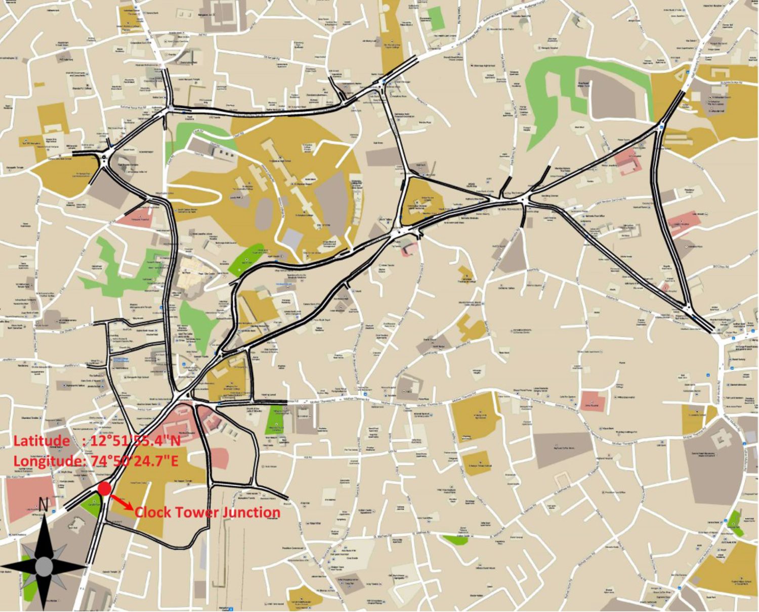
Mangalore is a beautiful scenic city in the southern part of the State of Karnataka, India. It is an emerging city located at 12°51'55.4" N latitude and 74°50'24.7" E longitude, at an altitude of 22 m above sea-level, and is well-connected by air, rail, and road. Mangalore City Corporation (MCC) witnessed an increase in population from 195,000 in 1971 to 488,968 in 2011 (Census, 2011) and is spread over 60 urban wards, covering an area of about 132.45 square km (MCC, 2015). The current population in the city is about 601173 (GoK, 2013), with a total road length of 1133.31km (MCC, 2016).
The heterogeneous mix of vehicles in the city includes cars, light commercial vehicles (LCVs) with a gross vehicle weight of lesser than 7.5 metric tons, buses, auto-rickshaws, and motorized two-wheelers. The average annual increase in the total number of vehicles during 2012-18 was about 10.86%, while the total vehicle count stood at 676,920 in March 2018. Presently, the percentage of cars, motorized two-wheelers, auto-rickshaws, LCVs, buses, and trucks comprise 19%, 71%, 4%, 2%, 1%, and 3% (GoK, 2018).
4. Data Collection
The present study included 423 links of road network spanning over 3.08 square km of Mangalore city connecting major junctions such as Hampankatta, Navbharat, PVS, Bunt’s Hostel, Jyothi, Bendoorwell, Balmatta, and St. Theresa’s School Junction. A few of these junctions are provided with fixed time traffic signals with manual override options to handle peak-hour traffic, while a majority of the junctions are manually controlled.
Video-graphic data on vehicular movements at eight major traffic junctions of the city and at 18 important mid-block sections of the road network were recorded for the peak-hour between 17.30-18.30 hours, during 10-18 March 2015 on mid-week days. A net total of 16-minutes peak-hour data was considered for the development of VISSIM model. A 12-minute video-graphic data that constitutes 75% of the data was used for testing, development, and calibration of VISSIM model, while a four-minute video-graphic data that constitutes 25% of the data was used for model validation.
As part of data collection efforts, additional video-graphic recordings of vehicular movements were used to determine the approximate speeds of randomly selected vehicles on selected road sections of the city. The acceleration values were also computed based on the initial and final speeds on road sections. It was proposed to use part of this information in assigning the desired speed distributions and the desired acceleration distributions.
4.1. Selection of Vehicle and Driver Characteristics and the Value Ranges for Preparation of Datasets
VISSIM comprises fifty vehicle and driver characteristics that can be refined and provides default values for the same. These vehicle and driver related characteristics can be simulated in various stages using a Monte Carlo approach or based on a deterministic simulation approach (Astarita and Giofré, 2019).
In a Monte Carlo based approach, the vehicle and driver characteristics to be tested are randomly generated. Park and Schneeberger (2003) adopted the Latin-Hypercube (LH) method of sampling for preparation of the datasets and evaluated 54 or 625 combinations of datasets considering 4 parameters and 5 value ranges. This approach can be considered similar to a stratified Monte Carlo sampling method where pairwise comparisons can be minimized.
The present study focuses on calibration of 14 vehicle and driver characteristics according to Wiedemann-74 (1974) car-following model over 14 operating value ranges. The vehicle types adopted in the present study include vehicles such as buses, cars, motorized two-wheelers, auto-rickshaws, and LCVs operating on Indian roads. The calibration of these vehicle and driver characteristics for a wide range of slow and fast motorized vehicles necessitates the use of a larger dataset where many more combinations of data need to be simulated. Due to this reason, it was considered ideal to adopt a deterministic simulation approach focusing on a smaller set of data. Moreover, it was proposed to study the accuracy of predictions when one of the vehicle and driver characteristics are varied so that it would enable the ANN-based module to effectively determine the sensitivity of each of the characteristics with respect to the other.
The data related to operating ranges of vehicle characteristics such as the distributions for the desired speed: lower bound, desired speed: upper bound, desired acceleration, maximum acceleration, and deceleration for each vehicle type used in India were specified in this study based on previous studies conducted by Mathew and Radhakrishnan (2010), Arasan and Krishnamurthy (2008), Manjunatha et al. (2013), Bains et al. (2013), and Mehar et al. (2014).
The operating ranges for driver characteristics related to minimum lateral clearance were arrived at based on Arasan and Krishnamurthy (2008), Manjunatha et al. (2013), and Bains et al. (2013) while the same for average standstill distance, minimum look-ahead distance, and minimum look-back distance were adopted based on previous studies performed by Mathew and Radhakrishnan (2010) and Siddharth and Ramadurai (2013).
The operating value ranges for minimum collision time-gain (or reaction time required to avoid collision while performing lateral movements), minimum longitudinal speed likely to be maintained for lane-change, additive and multiplicative part of desired safety distances between two vehicles, and time-between direction changes (for overtaking procedures) were assigned in the present study based on informal in-vehicle surveys with vehicle drivers in the city. Table 1 provides details on the operating value ranges for 14 vehicle and driver characteristics for the multi-stage first-level of calibrations performed in 14 major stages and 4 sub-stages involving 90 best performing simulation runs.
Suggested Lower and Upper Bound Values for Vehicle and Driver Characteristics Used in Performing Simulation Trials in VISSIM.
| Sl. No. | Vehicle and Driver Characteristics | Operating Value Range | Best performing simulation runs |
|---|---|---|---|
| 1 | Minimum Lateral Clearance (m) | 0.25 - 1.0 | 5 |
| 2a | Distributions for Desired Acceleration (m/s2) | 0.5 - 4.4 | 5 |
| 2b | Distributions for Maximum Acceleration (m/s2) | 1.0 - 4.4 | 5 |
| 2c | Distributions for Deceleration (m/s2) | 2.5 - 8.0 | 5 |
| 3a | Distributions for Desired Acceleration (m/s2) | 0.5 - 4.4 | 5 |
| 3b | Distributions for Maximum Acceleration (m/s2) | 1.0 - 4.4 | 5 |
| 4 | Minimum Look-ahead Distance (m) | 10 - 50 | 5 |
| 5 | Distributions for Maximum Acceleration (m/s2) | 1.0 - 4.4 | 5 |
| 6 | Distributions for Desired Acceleration (m/s2) | 0.5 - 4.4 | 5 |
| 7a | Distributions for Desired Speed (kmph) - Lower Bound | 21.9 - 72.3 | 5 |
| 7b | Distributions for Desired Speed (kmph) - Upper Bound | 21.9 - 72.3 | 5 |
| 8 | Minimum Look-back Distance (m) for car-following | 10.0 - 50.0 | 5 |
| 9 | Average Standstill Distance (m) for car-following | 0.5 - 2.5 | 5 |
| 10 | Additive Part of Desired Safety Distance (m) for car-following | 0.2 - 2.0 | 5 |
| 11 | Multiplicative Part of Desired Safety Distance (m) for car-following | 0.2 - 3.0 | 5 |
| 12 | Time-between Direction Changes (s) for overtaking | 1.0 - 10.0 | 5 |
| 13 | Minimum Longitudinal Speed (kmph) for lane change | 1.1 - 3.6 | 5 |
| 14 | Minimum Collision Time-gain for lateral driving behavior (s) | 0.40 - 2.0 | 5 |
| Total simulation runs in the first-level calibrations | 90 |
-
Source: Authors own creation.
5. Methodology Adopted in this Study
The following sub-sections provide descriptions on the methodology adopted in various phases of work undertaken in this study. Details on the creation of a high-resolution map of the city, prelimCinary steps in model development in VISSIM, measures of effectiveness adopted for the study, identification of the best random seed, first-level of calibrations, ANN-based sensitivity analysis, second-level of calibrations, and validation of the model are discussed below.
5.1. Creation of a High-resolution map for the city
An AutoCAD drawing with details on the road geometrics, widths of the road links, and dimensions of the junctions was prepared based on measurements made at various locations in the city. For the road-stretches of the city that remained unchanged for the past decade, the information contained in drawings prepared previously by Dalal Consultants and Engineers (2003) were used to update AutoCAD drawing in 2015.
Additionally, a high resolution .jpg digitized base-map (of 6284 x 6726-pixel size and 3.43MB size) of the city was developed to a scale of 1:5000. AutoCAD drawing prepared earlier in 2015 was then overlaid on the digitized base-map in AutoCAD, and re-aligned to ensure a perfect match. The .jpg base-map along with the re-aligned AutoCAD drawing was then saved as a composite .dwg image as shown in Figure 1.
AutoCAD Drawing Interfaced with High-Resolution Map of Mangalore City.
5.2. Preliminary steps in model development and measures of effectiveness
The composite .dwg file created in the previous step was then uploaded to VISSIM using the background option. This background was used as a template in VISSIM for drawing the links and connectors for the road network of the study area.
It was planned to adopt Wiedemann-74 (1974) car-following behavior for modeling driving behavior on urban roads with merging traffic in this study. The values for driver and vehicle characteristics were set to default values in VISSIM at the beginning of the simulation run.
As part of the preliminary steps in the model development exercise, it was also required to identify the best random seed from among commonly used random seeds for microsimulation using measures of effectiveness such as GEH statistic, RNSE, and mean absolute error (MAE) in the prediction of traffic volumes. The accuracy of prediction for traffic volumes at 18 mid-block sections spread over the city was used for this purpose. The expression for GEH statistic is given as (DMRB, 1996; Smith and Blewitt, 2010),
where, M is the hourly traffic volume predicted or simulated by the traffic model, and C is the observed hourly traffic count.
According to UKDoT (2014) and WSDoT (2014), GEH statistic value of lesser than 5.0 for atleast 85% of the road links calibrated is considered to provide a good fit in addition to the requirement that the individual link-flows must have a predictive accuracy of 15% in atleast 85% of the road links that have traffic flows between 700 and 2700 vehicles per hour.
Alternatively, the statistic RNSE (root normalized squared error), a modified form of GEH statistic is also used by various agencies including Wisconsin-DoT (2005). The RNSE statistic is expressed as,
5.3. Procedure adopted for identification of the best random seed for simulation
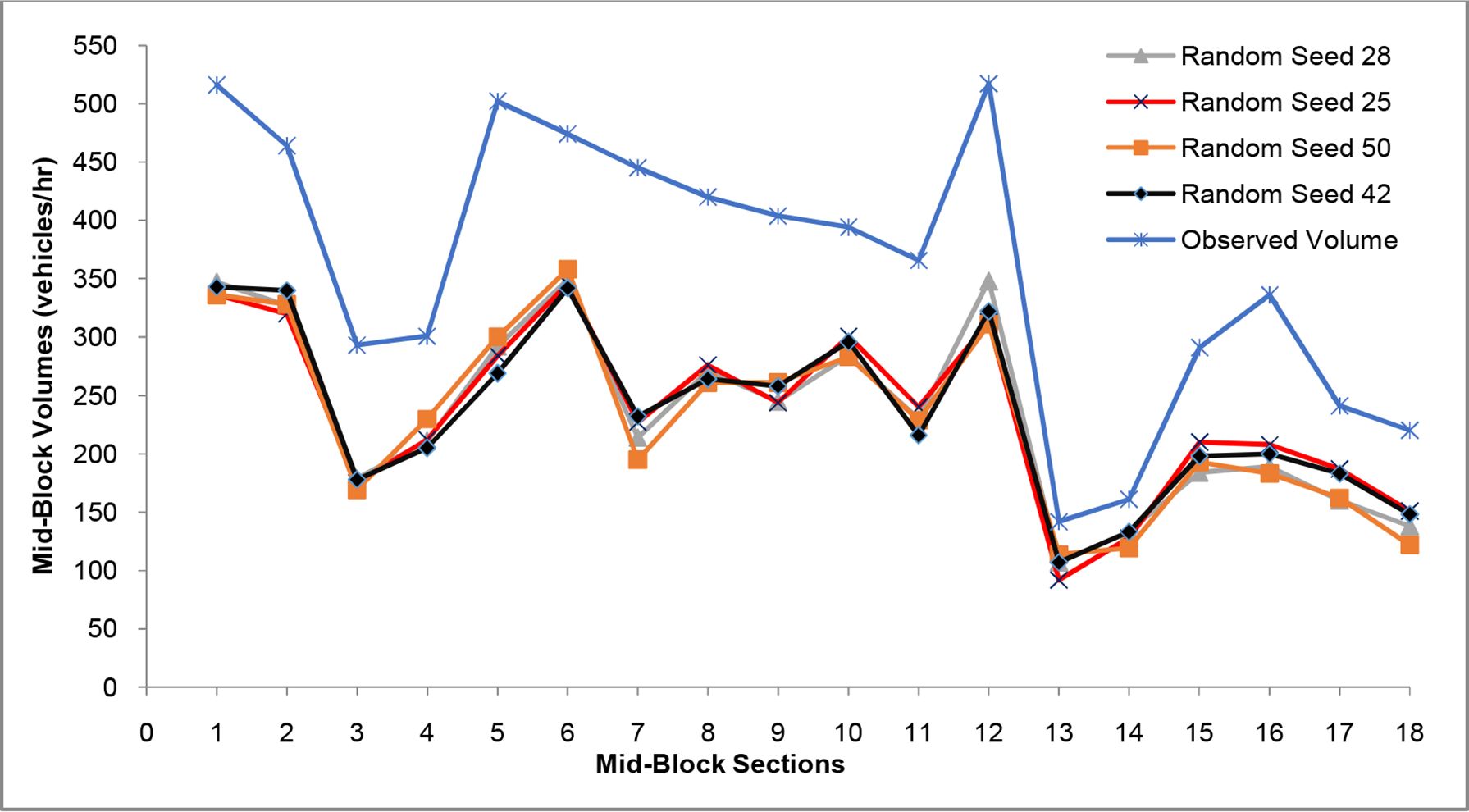
Preliminary trial runs using random seeds 1 to 50 were performed to identify the most ideal random seed for simulation as part of the present study. Here, it was observed that random seeds 25 and 42 provided lesser prediction errors for simulations in Mangalore city. Figure 2 illustrates details on the results of trials conducted using random seeds 25, 28, 42, and 50 where the mean absolute errors (MAE) in the prediction of traffic flows at 18 mid-block sections were found to be lower. Simulation experiments reported by various researchers (Wang et al., 2012; Ishaque and Noland, 2005; Kamdar, 2004; TJPDC, 2007; Arkatkar et al., 2016) based on numerous trials also indicate that the use of random numbers 25, 28, 42, and 50 provide reliable estimates of the actual values.
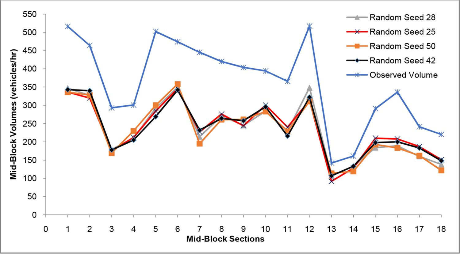
A Pictorial Representation of Observed and Predicted Volumes at 18 mid-block Sections Using Random Seeds 25, 28, 42, and 50.
The trial runs indicated that simulations using random seeds 42 and 25 resulted in lower mean absolute errors (MAE) of 33.4% and 33.4% respectively when simulated with default values in VISSIM. Also, the corresponding GEH statistic values were computed as 7.06 and 7.02 respectively for random seeds 42 and 25. However, the random seed 42 was used for calibrations since Wang et al. (2012) observed that the use of random seeds higher than 25 could result in lesser standard errors. PTV (2014) also recommends the use of random seed 42 especially in the studies related to predicting inter-arrival time of vehicles. Additionally, it was observed in the present study that performing trial runs for random seed greater than 50 resulted in higher prediction errors. In the light of the above references and also based on simulations performed for random seeds 1-50, it may be considered that the likely set of best performing random variables has been evaluated. Thus, the selection of random seed and the calibration of vehicle and driver characteristics are based on a deterministic approach in this study. Liu (2002) too recommends that simulation trials may be performed using a selected set of random seeds in order to achieve the desired results. A similar approach has been adopted in this study.
On the other hand, Monte Carlo simulations depend upon the use of random numbers to identify a set of stochastic combinations of characteristics to be tested (Newman and Barkema, 1999). But such approaches are found to be useful in situations where the number of characteristics to be evaluated and the value ranges are within reasonable limits (Mattis, 1976). Also, the results obtained using Monte Carlo approaches may not be reliable or may involve more number of trials according to Park and Miller (1988).
5.4. The multi-stage first-level of calibrations
As part of the multi-stage first-level of calibrations, fine-tuning of vehicle and driver characteristics was performed in 14 major stages with sub-stages in the 2nd, 3rd, and the 7th stages. The sequence of selection of characteristics to be refined or fine-tuned in each stage was arrived at based on a number of informal trial runs. The calibrations were performed in a manner to ensure that the accuracy of predicting traffic volumes at 18 mid-blocks of the city improved when measured based on the mean absolute error, GEH statistic, and RNSE. The details on various stages of refinement for the vehicle and driver characteristics are summarized below:
Stage 1 - Assigning minimum lateral clearances between vehicles for various vehicle types.
Stage 2a - Assigning acceptable desired acceleration distributions for various vehicle types.
Stage 2b - Assigning acceptable maximum acceleration distributions for various vehicle types.
Stage 2c - Assigning acceptable deceleration distributions for various vehicle types.
Stage 3a - First series of Refinement in the acceptable desired acceleration distributions for various vehicle types.
Stage 3b - First series of Refinement in the acceptable maximum acceleration distributions for various vehicle types.
Stage 4 - Assigning minimum look-ahead distances for each vehicle type as part of car-following characteristics.
Stage 5 - Second series of refinement in the maximum acceleration distributions for various vehicle types.
Stage 6 - Second series of refinement in the desired acceleration distributions for various vehicle types.
Stage 7a - Assigning desired speed: lower bounds for speed distributions of each vehicle type.
Stage 7b - Assigning desired speed: upper bounds for speed distributions of each vehicle type.
Stage 8 - Assigning minimum look-back distances as part of car-following characteristics for various vehicle types.
Stage 9 - Assigning average standstill distances as part of car-following characteristics for various vehicle types.
Stage 10 - Refining the value of additive part of desired safety distance as part of car-following characteristics for various vehicle types.
Stage 11 - Refining the value of multiplicative part of desired safety distance as part of car-following characteristics for various vehicle types.
Stage 12 - Assigning values of time-between direction changes for overtaking for various vehicle types.
Stage 13 - Refining the value of minimum longitudinal speed as part of lane change behavior for various vehicle types.
Stage 14 - Refinement of minimum collision time-gain as part of lateral driving behavior for various vehicle types.
The details on the changes made to each of the vehicle and driver characteristics at each of the best performing simulation runs, along with the corresponding mean absolute errors (MAE) were provided as an input to ANN-based sensitivity analysis module. This approach was considered to be ideal in the present study as it would enable the ANN to easily identify the relative importance or sensitivity of each of the characteristics with respect to the other.
5.5. Approach to sensitivity analysis of vehicle and driver characteristics
Sensitivity analysis assists in evaluating the efficacy of various strategies adopted on the predictive capability of the model. This will further help in understanding the relative influence of various vehicle and driver characteristics on the performance of the model. The results of the sensitivity analysis can be used in the second-level of calibrations in order to fine-tune the model.
Traditionally, in elasticity-based approaches, sensitivity is measured as the ratio between the change in the dependent variable (or the value of the final objective function) and the change in the value of an independent variable (or the value of a chosen characteristic). Sensitivity can thus be expressed as,
In the present study, ANN-based approach was considered for the analysis of sensitivity as ANNs are capable of capturing the underlying relationships more effectively when compared to other approaches (Lippmann, 1987; Scarborough and Somers, 2006; Dreiseitl and Ohno-Machado, 2002; WiscCS, 1989).
Rao et al. (1998) adopted ANN-based approach for assessing the sensitivity of various input variables in mode-choice modeling, where the weight-partition method as explained by Garson (1991) was used. Here, it was observed that the results obtained were almost similar to those determined using the multinomial logit model (MNL) approach.
Kalteh (2008) adopted a similar approach in the study of relative importance of variables that contributed to the prediction of rainfall-runoff using ANN. Feng et al. (2011) too observed that Garson’s algorithm could be used in identifying the variables that influenced route-choice selection that resulted in predictions close to 97.4% accuracy. Shafabakhsh et al. (2015) adopted the above approach in the determination of factors influencing the thickness of pavements. However, the application of such approaches in the field of microsimulation and traffic engineering seems to be limited.
The Garson’s algorithm (1991) has been observed to be widely adopted in determining the relative importance of input variables for ANN structures with a single hidden layer in addition to the alternative approaches recommended by Gevrey et al., 2003; Gevrey et al., 2006 and Olden and Jackson (2002). Özesmi and Özesmi (1999) suggested a more robust approach that could handle complex ANN structures with one, two or more hidden layers.
Equation (4) provides details on the formulae adopted in computing the relative importance of input variables based on the method recommended by Özesmi and Özesmi (1999). It is observed that a similar approach is adopted in the computations made as part of the EasyNN-plus software.
where, Ri = relative importance (%) of the ith neuron representing the ith input variable; = importance of the ith input variable when computed considering outputs to the jth neuron in the hidden layer; Wi,j = connection weight from the ith input neuron to the jth hidden neuron; n = number of input neurons representing the input variables; m = number of neurons in the hidden layer.
In other words, according to Özesmi and Özesmi (1999), the relative importance of the input variable is equal to the sum of squares of connection weights destined to other neurons from the ith input variable, divided by the sum of squares of such weights for all the input variables. The present study proposes the application of this approach for the measurement of sensitivity (or the relative importance of vehicle and driver characteristics).
5.5.1. Preparation of datasets for ANN-based sensitivity analysis
Based on the simulations performed in the first-level of calibrations as explained in the above sections, information on the changes made to the vehicle and driver characteristics and the corresponding changes in the mean absolute errors (MAE) over 91 calibration runs including the first simulation run with default values and the simulation runs for the 14 major stages and the sub-stages were tabulated.
The values tabulated for the 91 rows of data were then normalized based on the minimum and maximum value ranges to lie between 0 and 1 respectively. Here, it may be observed that although the simulations were performed by assigning different values for the desired speed: lower and upper bounds for speed distributions for various vehicle types, only the weighted average of the values were used while tabulating the data. In this connection, it may be noted that the percentages of motorized two-wheelers, auto-rickshaws, trucks, cars, buses, and LCVs in the road network were 47.3%, 18.1%, 0.2%, 27%, 5.8%, and 1.6% respectively. A partial listing of the normalized database used for training the ANN model is provided in Table 2.
A Partial Listing of the Normalized Database Used for Training the ANN Model.
| Details on Data Set for Sensitivity Analysis for Vehicle and Driver Characteristics | |||||||||||||||
|---|---|---|---|---|---|---|---|---|---|---|---|---|---|---|---|
| First-level of Calibration Stage Sl. No. | Minimum Lateral Clearances (m) | Desired Accelerations at Desired Speed of 50 kmph (m/s2) | Maximum Accelerations at Desired Speed of 50 kmph (m/s2) | Deceleration Distribution (m/s2) | Weighted Average of Speed Distribution Lower-Bounds (kmph) | Weighted Average of Speed Distribution Upper-Bounds (kmph) | Minimum Look-ahead Distances (m) | Minimum Look-back Distances (m) | Average Standstill Distances (m) | Additive Part of Desired Safety Distances (m) | Multiplicative Part of Desired Safety Distances (m) | Time-Between Direction Changes (s) | Minimum Longitudinal Speeds (kmph) | Minimum Collision Time-gains (s) | Mean Absolute Errors (%) |
| (1) | (2) | (3) | (4) | (5) | (6) | (7) | (8) | (9) | (10) | (11) | (12) | (13) | (14) | (15) | (16) |
| Ini--tial | 1.00 | 0.432 | 0.432 | 0.335 | 0.96 | 0.69 | 0.20 | 0.20 | 0.80 | 1.00 | 1.00 | 0.10 | 1.00 | 1.00 | 0.9653 |
| 1 | 0.50 | 0.432 | 0.432 | 0.335 | 0.96 | 0.69 | 0.20 | 0.20 | 0.80 | 1.00 | 1.00 | 0.10 | 1.00 | 1.00 | 0.9653 |
| 0.25 | 0.432 | 0.432 | 0.335 | 0.96 | 0.69 | 0.20 | 0.20 | 0.80 | 1.00 | 1.00 | 0.10 | 1.00 | 1.00 | 0.9653 | |
| 0.75 | 0.432 | 0.432 | 0.335 | 0.96 | 0.69 | 0.20 | 0.20 | 0.80 | 1.00 | 1.00 | 0.10 | 1.00 | 1.00 | 0.9653 | |
| 0.65 | 0.432 | 0.432 | 0.335 | 0.96 | 0.69 | 0.20 | 0.20 | 0.80 | 1.00 | 1.00 | 0.10 | 1.00 | 1.00 | 0.9653 | |
| 0.85 | 0.432 | 0.432 | 0.335 | 0.96 | 0.69 | 0.20 | 0.20 | 0.80 | 1.00 | 1.00 | 0.10 | 1.00 | 1.00 | 0.9653 | |
| 2a | 0.50 | 0.159 | 0.432 | 0.335 | 0.96 | 0.69 | 0.20 | 0.20 | 0.80 | 1.00 | 1.00 | 0.10 | 1.00 | 1.00 | 0.9653 |
| 0.50 | 0.295 | 0.432 | 0.335 | 0.96 | 0.69 | 0.20 | 0.20 | 0.80 | 1.00 | 1.00 | 0.10 | 1.00 | 1.00 | 0.9653 | |
| 0.50 | 0.409 | 0.432 | 0.335 | 0.96 | 0.69 | 0.20 | 0.20 | 0.80 | 1.00 | 1.00 | 0.10 | 1.00 | 1.00 | 0.9653 | |
| 0.50 | 0.455 | 0.432 | 0.335 | 0.96 | 0.69 | 0.20 | 0.20 | 0.80 | 1.00 | 1.00 | 0.10 | 1.00 | 1.00 | 0.9653 | |
| 0.50 | 0.114 | 0.432 | 0.335 | 0.96 | 0.69 | 0.20 | 0.20 | 0.80 | 1.00 | 1.00 | 0.10 | 1.00 | 1.00 | 0.9653 | |
| 2b | 0.50 | 0.159 | 0.295 | 0.335 | 0.96 | 0.69 | 0.20 | 0.20 | 0.80 | 1.00 | 1.00 | 0.10 | 1.00 | 1.00 | 0.9653 |
| 0.50 | 0.159 | 0.568 | 0.335 | 0.96 | 0.69 | 0.20 | 0.20 | 0.80 | 1.00 | 1.00 | 0.10 | 1.00 | 1.00 | 0.9653 | |
| 0.50 | 0.159 | 0.705 | 0.335 | 0.96 | 0.69 | 0.20 | 0.20 | 0.80 | 1.00 | 1.00 | 0.10 | 1.00 | 1.00 | 0.9653 | |
| 0.50 | 0.159 | 0.705 | 0.335 | 0.96 | 0.69 | 0.20 | 0.20 | 0.80 | 1.00 | 1.00 | 0.10 | 1.00 | 1.00 | 0.9653 | |
| 0.50 | 0.159 | 0.250 | 0.335 | 0.96 | 0.69 | 0.20 | 0.20 | 0.80 | 1.00 | 1.00 | 0.10 | 1.00 | 1.00 | 0.9653 | |
| 2c | 0.50 | 0.159 | 0.295 | 0.334 | 0.96 | 0.69 | 0.20 | 0.20 | 0.80 | 1.00 | 1.00 | 0.10 | 1.00 | 1.00 | 0.9653 |
| 0.50 | 0.159 | 0.295 | 0.675 | 0.96 | 0.69 | 0.20 | 0.20 | 0.80 | 1.00 | 1.00 | 0.10 | 1.00 | 1.00 | 0.9653 | |
| 0.50 | 0.159 | 0.295 | 0.738 | 0.96 | 0.69 | 0.20 | 0.20 | 0.80 | 1.00 | 1.00 | 0.10 | 1.00 | 1.00 | 0.9653 | |
| 0.50 | 0.159 | 0.295 | 1.000 | 0.96 | 0.69 | 0.20 | 0.20 | 0.80 | 1.00 | 1.00 | 0.10 | 1.00 | 1.00 | 0.9653 | |
| 0.50 | 0.159 | 0.295 | 0.313 | 0.96 | 0.69 | 0.20 | 0.20 | 0.80 | 1.00 | 1.00 | 0.10 | 1.00 | 1.00 | 0.9653 | |
| - | - | - | - | - | - | - | - | - | - | - | - | - | - | - | - |
| 13 | 0.50 | 0.341 | 0.341 | 0.334 | 0.61 | 0.86 | 0.80 | 0.60 | 0.40 | 0.20 | 0.17 | 0.50 | 0.53 | 1.00 | 0.2948 |
| 0.50 | 0.341 | 0.341 | 0.334 | 0.61 | 0.86 | 0.80 | 0.60 | 0.40 | 0.20 | 0.17 | 0.50 | 0.83 | 1.00 | 0.3295 | |
| 0.50 | 0.341 | 0.341 | 0.334 | 0.61 | 0.86 | 0.80 | 0.60 | 0.40 | 0.20 | 0.17 | 0.50 | 0.67 | 1.00 | 0.3295 | |
| 0.50 | 0.341 | 0.341 | 0.334 | 0.61 | 0.86 | 0.80 | 0.60 | 0.40 | 0.20 | 0.17 | 0.50 | 0.42 | 1.00 | 0.3035 | |
| 0.50 | 0.341 | 0.341 | 0.334 | 0.61 | 0.86 | 0.80 | 0.60 | 0.40 | 0.20 | 0.17 | 0.50 | 0.31 | 1.00 | 0.3064 | |
| 14 | 0.50 | 0.341 | 0.341 | 0.334 | 0.61 | 0.86 | 0.80 | 0.60 | 0.40 | 0.20 | 0.17 | 0.50 | 0.53 | 0.29 | 0.2775 |
| 0.50 | 0.341 | 0.341 | 0.334 | 0.61 | 0.86 | 0.80 | 0.60 | 0.40 | 0.20 | 0.17 | 0.50 | 0.53 | 0.20 | 0.2948 | |
| 0.50 | 0.341 | 0.341 | 0.334 | 0.61 | 0.86 | 0.80 | 0.60 | 0.40 | 0.20 | 0.17 | 0.50 | 0.53 | 0.40 | 0.3006 | |
| 0.50 | 0.341 | 0.341 | 0.334 | 0.61 | 0.86 | 0.80 | 0.60 | 0.40 | 0.20 | 0.17 | 0.50 | 0.53 | 0.75 | 0.3266 | |
| 0.50 | 0.341 | 0.341 | 0.334 | 0.61 | 0.86 | 0.80 | 0.60 | 0.40 | 0.20 | 0.17 | 0.50 | 0.53 | 0.55 | 0.2861 | |
-
Source: Authors own creation.
5.5.2. Determination of the ideal configuration for ANN model
The above-mentioned database with normalized values was used to train the ANN using EasyNN-plus software. ANN model was initially formulated with 14 neurons in the input layer to represent 14 vehicle and driver characteristics, 15 neurons in a single hidden layer, and 1 neuron in the output layer to represent the mean absolute error in simulation. ANN was required to learn the pattern of distribution of mean absolute errors for the 91 rows of normalized data.
The difference between the modeled error-values predicted using ANN and the actual mean absolute errors given as input were required to be lesser by specifying a target error of lesser than 0.1 for all the rows of dataset in EasyNN-plus software. Additionally, the maximum number of training cycles was set to 50,000. The software automatically optimized the learning rate to 0.7 and momentum to 0.8 in the training phase in this study.
In the later stages, an ANN was tested for various configurations by altering the number of neurons in the hidden layers, and also by varying the number of hidden layers in order to determine the ideal configuration. Details on the tests performed using EasyNN-plus for various configurations of ANN are provided in Table 3 along with the prediction errors and number of training cycles taken for convergence.
Details on Tests for Identifying the Ideal ANN Configuration.
| Test Serial No. | Number of Neurons in the Hidden Layers | Mean Absolute Error (MAE) in Prediction(%) | Number of training cycles for convergence | ||
|---|---|---|---|---|---|
| HiddenLayerNo: 1 | HiddenLayerNo: 2 | HiddenLayerNo: 3 | |||
| 1 | 15 | 0 | 0 | 3.8075 | 10751 |
| 2 | 14 | 0 | 0 | 3.7303 | 11407 |
| 3 | 13 | 0 | 0 | 3.9456 | 10276 |
| *4 | 12 | 0 | 0 | 3.0979 | 11184 |
| 5 | 11 | 0 | 0 | 3.7925 | 11265 |
| 6 | 10 | 0 | 0 | 3.4415 | 10138 |
| 7 | 9 | 0 | 0 | 3.2023 | 11312 |
| 8 | 8 | 0 | 0 | 3.7263 | 10015 |
| 9 | 7 | 0 | 0 | 3.4304 | 10864 |
| 10 | 6 | 0 | 0 | 3.7916 | 10319 |
| 11 | 5 | 0 | 0 | 3.7277 | 9677 |
| 12 | 4 | 0 | 0 | 3.7169 | 6234 |
| 13 | 12 | 12 | 0 | 3.6959 | 5407 |
| 14 | 12 | 11 | 0 | 3.4819 | 4803 |
| 15 | 12 | 10 | 0 | 3.8747 | 3468 |
| 16 | 12 | 9 | 0 | 3.8354 | 6072 |
| *17 | 12 | 8 | 0 | 3.4290 | 4021 |
| 18 | 12 | 7 | 0 | 3.4600 | 3548 |
| 19 | 12 | 6 | 0 | 3.6131 | 2984 |
| 20 | 12 | 5 | 0 | 4.3240 | 1353 |
| 21 | 12 | 4 | 0 | 3.9310 | 4506 |
| 22 | 12 | 3 | 0 | 5.4365 | 1231 |
| 23 | 12 | 2 | 0 | 5.3433 | 4619 |
| 24 | 12 | 8 | 8 | 3.5013 | 6229 |
| 25 | 12 | 8 | 7 | 3.0347 | 7672 |
| 26 | 12 | 8 | 6 | 3.5135 | 9181 |
| 27 | 12 | 8 | 5 | 4.2408 | 2670 |
| *28 | 12 | 8 | 4 | 2.9404 | 5261 |
| 29 | 12 | 8 | 3 | 4.0352 | 2314 |
| 30 | 12 | 8 | 2 | 3.0703 | 16403 |
| 31 | 12 | 8 | 1 | 4.4979 | 3347 |
-
Source: Authors own creation.
-
Note: *Optimum ANN configurations for neurons organized in 1, 2, or 3 hidden layers. Target error = 0.1; Learning rate = 0.7; Momentum rate = 0.8; Number of neurons in the input layer = 14; Number of neurons in the output layer = 1.
Here, it can be found that the ideal configuration for ANN model comprises 14 neurons in the input layer, 12, 8, and 4 neurons respectively in the first, second, and the third hidden layers and one neuron in the output layer. For this configuration, the mean absolute error for ANN was found to be a minimum of 2.94% when ANN was trained for 5261 cycles.
5.6. The three-stage second-level of calibration
As part of the second-level of calibrations, driver characteristics such as the average standstill distance and the minimum look-ahead distance, and the vehicle characteristic of desired speed: lower bounds were fine-tuned in three major stages over a total of 45 simulation runs aimed at achieving better predictions of traffic volumes.
5.7. Model validation
The best vehicle and driver characteristics identified based on the first-level of calibrations, along with the refinements made in the second-level of calibrations were used in validating the VISSIM model. The validation exercise was performed on 25% of the video-graphic data recorded for 18 mid-block sections of the city.
6. Results and Discussions on Calibration, Sensitivity Analysis, and Validation
The following sub-sections provide details on the results of the first-level of calibrations (performed in 14 major stages), sensitivity analysis, the second-level of calibrations (performed in three major stages), and the validation of simulation model.
6.1. Results and discussions on the first-level of calibrations
An initial test-run using random seed 42 which was identified as the best random seed was performed in VISSIM with default values assigned to the vehicle and driver characteristics. A number of informal trial runs were conducted by fine-tuning vehicle and driver characteristics before commencing the first-level of calibrations. The best sequence of refinement of various vehicle and driver characteristics was then evolved using a trial and error approach.
In Stage 1 of the first-level of calibrations, the minimum lateral clearance for each type of vehicle was assigned based on the recommendations provided by Arasan and Krishnamurthy (2008), Manjunatha et al. (2013), and Bains et al. (2013). In Stages 2a, 2b, and 2c of refinement, the values associated with the distributions for desired accelerations, maximum accelerations, and decelerations respectively were set for each vehicle-type as a part of refining vehicle characteristics using a trial and error method considering values adopted and modified based on Arasan and Krishnamurthy (2008). After these stages of refinements, the mean absolute error remained stable at around 33.4% and the GEH statistic also remained unchanged at 7.06.
In Stages 3a and 3b, the distributions for desired accelerations and maximum accelerations respectively were refined as a part of vehicle characteristics considering values adopted and modified based on Mathew and Radhakrishnan (2010), Mehar et al. (2014), and Bains et al. (2013). Through these refinements, the mean absolute error reduced from 33.4% to 32.9% and the GEH statistic decreased marginally from 7.06 to 6.94.
In Stage 4, the value associated with the minimum look-ahead distance was assigned as part of driver characteristics and the best value for vehicles plying on the city roads was identified as 40m. The mean absolute error at this stage reduced from 32.9% to 29.5% and the GEH statistic reduced significantly from 6.94 to 6.14 indicating that the assigned value improved significantly.
In Stage 5, the values associated with the distributions for maximum accelerations were further refined to increase the accuracy of prediction. At this stage, the mean absolute error reduced from 29.5% to 27.5%, and the GEH statistic reduced from 6.14 to 5.82. In Stage 6, the values associated with the distributions for desired accelerations were further refined to tally with the actual on-field acceleration conditions. Here, the mean absolute error reduced slightly from 27.5% to 27.2%, and the GEH statistic showed a minor reduction from 5.82 to 5.63.
In Stages 7a and 7b of refinement, the values related to the desired speed: lower and upper bounds for speed distributions of various vehicle types were assigned considering values adopted and modified based on Arasan and Krishnamurthy (2008). In these stages, the mean absolute error reduced from 27.2% to 24.5%, and the GEH statistic showed a reduction from 5.63 to 5.12, signifying a moderate improvement in the prediction of traffic volumes.
In Stage 8, the value associated with the minimum look-back distance was assigned as part of fine-tuning driver characteristics. At this stage, the best value for the minimum look-back distance of 30m was arrived at for vehicles plying on the city roads. The mean absolute error reduced from 24.5% to 22.4%, and the GEH statistic reduced from 5.12 to 4.65.
In Stage 9, the value related to the average standstill distance was assigned as part of driver characteristics and the best value for vehicles plying on the city roads was identified as 1m. The mean absolute error reduced from 22.4% to 20.1% and the GEH statistic reduced from 4.65 to 4.08. In Stage 10, the additive part of desired safety distance was refined to 0.4m as part of fine-tuning driver characteristics. At this stage, the mean absolute error reduced from 20.1% to 13.8% and the GEH statistic reduced from 4.08 to 2.74, showing a significant improvement in the accuracy of predictions.
In Stage 11 of refinement, the multiplicative part of desired safety distance was refined to 0.5m as part of fine-tuning driver characteristics. Here, the mean absolute error was found to reduce from 13.8% to 10.3% and the GEH statistic displayed a significant reduction from 2.74 to 2.0. In Stage 12, the time-between direction changes was refined to 5seconds as part of fine-tuning driver characteristics. The mean absolute error was found to be unchanged at around 10.3% while the GEH statistic reduced slightly from 2.05 to 2.01.
In Stage 13, the minimum longitudinal speed (required for lateral movement) was refined to 1.9kmph as part of fine-tuning driver characteristics. The mean absolute error reduced from 10.3% to 10.2% and the GEH statistic reduced from 2.0 to 1.97.
Finally, in Stage 14 of refinement, the minimum collision time-gain was fine-tuned to 0.57 seconds as part of driver characteristics. The mean absolute error reduced from 10.2% to 9.6% and the GEH statistic reduced from 1.97 to 1.89 as in Table 4 for the final stage of refinement.
Details of MAE, GEH, and RNSE at 18 Mid-Block Sections after Stage 14 of First-Level of Calibrations.
| Direction of Traffic Flow | Simulated volume | Observed volume | Absolute Error (%) | GEH Statistic | RNSE Statistic | |
|---|---|---|---|---|---|---|
| From | To | |||||
| Jyothi | Hampankatta | 465 | 516 | 9.9 | 2.30 | 2.25 |
| Hampankatta | Jyothi | 431 | 464 | 7.1 | 1.56 | 1.53 |
| PVS | Bunts | 282 | 293 | 3.8 | 0.65 | 0.64 |
| Bunts | PVS | 239 | 301 | 20.6 | 3.77 | 3.57 |
| Navabharat | PVS | 441 | 502 | 12.2 | 2.81 | 2.72 |
| PVS | Navabharat | 464 | 474 | 2.1 | 0.46 | 0.46 |
| Hampankatta | Navabharat | 382 | 445 | 14.2 | 3.10 | 2.99 |
| Navabharat | Hampankatta | 357 | 420 | 15.0 | 3.20 | 3.07 |
| Jyothi | Bunts | 343 | 404 | 15.1 | 3.16 | 3.03 |
| Bunts | Jyothi | 378 | 394 | 4.1 | 0.81 | 0.81 |
| Jyothi | Balmatta | 315 | 366 | 13.9 | 2.76 | 2.67 |
| Balmatta | Jyothi | 476 | 517 | 7.9 | 1.84 | 1.80 |
| Balmatta | St. Theresa | 132 | 142 | 7.0 | 0.85 | 0.84 |
| St. Theresa | Balmatta | 174 | 161 | 8.1 | 1.00 | 1.02 |
| Bendoorwell | Balmatta | 270 | 291 | 7.2 | 1.25 | 1.23 |
| Balmatta | Bendoorwell | 275 | 336 | 18.2 | 3.49 | 3.33 |
| Bendoorwell | St. Theresa | 241 | 241 | 0.0 | 0.00 | 0.00 |
| St. Theresa | Bendoorwell | 205 | 220 | 6.8 | 1.03 | 1.01 |
| MAE | 9.6 | 1.89 | 1.83 | |||
-
Source: Authors own creation.
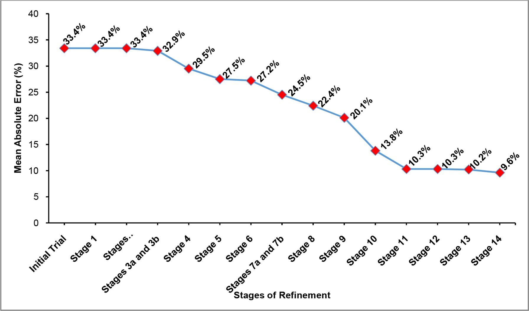
Table 5 provides a summary of the mean absolute errors and the values of the mean GEH statistic at each stage of refinement in the calibration procedure, while Figure 3 provides a pictorial representation of the same. The summary of the values of vehicle and driver characteristics at the end of the first-level of calibrations are provided in Table 6.
Summary of the MAE and the GEH at each Stage of Refinement in the First-Level of Calibrations.
| Stages of Refinement | Mean Absolute Errors at the end of the stages (%) | Mean GEH Statistic |
|---|---|---|
| Initial trial (default value) | 33.4 | 7.06 |
| Stage 1 | 33.4 | 7.06 |
| Stages 2a, 2b, and 2c | 33.4 | 7.06 |
| Stages 3a and 3b | 32.9 | 6.94 |
| Stage 4 | 29.5 | 6.14 |
| Stage 5 | 27.5 | 5.82 |
| Stage 6 | 27.2 | 5.63 |
| Stages 7a and 7b | 24.5 | 5.12 |
| Stage 8 | 22.4 | 4.65 |
| Stage 9 | 20.1 | 4.08 |
| Stage 10 | 13.8 | 2.74 |
| Stage 11 | 10.3 | 2.05 |
| Stage 12 | 10.3 | 2.01 |
| Stage 13 | 10.2 | 1.97 |
| Stage 14 | 9.6 | 1.89 |
-
Source: Authors own creation.
Summary of Values of Vehicle and Driver Characteristics at the End of First and Second-Levels of Calibrations.
| Sl. No. | Vehicle and Driver Characteristics | Calibrated Value | |||||
|---|---|---|---|---|---|---|---|
| Car | MTW | Auto-rickshaw | LCV | Bus | Truck | ||
| Vehicle and Driver Characteristics at the End of First Level of Calibrations | |||||||
| 1 | Minimum Lateral Clearances (m) | 0.5 | 0.5 | 0.5 | 0.5 | 0.5 | 0.5 |
| 2 | Desired Accelerations at 50kmph (m/s2) | 1.7 | 1.6 | 0.5 | 0.7 | 0.5 | 0.4 |
| 3 | Maximum Accelerations at 50kmph (m/s2) | 1.8 | 1.7 | 0.6 | 0.8 | 0.7 | 0.7 |
| 4 | Deceleration Distributions (m/s2) | 2.8 | 2.8 | 2.4 | 2.1 | 2.2 | 1.8 |
| 5 | Desired Speed: Lower Bounds (kmph) | 35 | 30 | 30 | 38 | 37 | 30 |
| 6 | Desired Speed: Upper Bounds (kmph) | 70 | 60 | 55 | 68 | 65 | 60 |
| 7 | Minimum Look-ahead distances (m) | 40 | 40 | 40 | 40 | 40 | 40 |
| 8 | Minimum Look-back distances (m) | 30 | 30 | 30 | 30 | 30 | 30 |
| 9 | Average Stand Still Distances (m) | 1.0 | 1.0 | 1.0 | 1.0 | 1.0 | 1.0 |
| 10 | Additive Part of Desired Safety Distances (m) | 0.4 | 0.4 | 0.4 | 0.4 | 0.4 | 0.4 |
| 11 | Multiplicative Part of Desired Safety Distances (m) | 0.5 | 0.5 | 0.5 | 0.5 | 0.5 | 0.5 |
| 12 | Time-Between Direction Changes (s) | 5.0 | 5.0 | 5.0 | 5.0 | 5.0 | 5.0 |
| 13 | Minimum Longitudinal Speeds (kmph) | 1.9 | 1.9 | 1.9 | 1.9 | 1.9 | 1.9 |
| 14 | Minimum Collision Time-gains (s) | 0.57 | 0.57 | 0.57 | 0.57 | 0.57 | 0.57 |
| Vehicle and Driver Characteristics Revised at the End of Second Level of Calibrations | |||||||
| 1 | Average Stand Still Distance (m) | 0.4 | 0.4 | 0.4 | 0.4 | 0.4 | 0.4 |
| 2 | Minimum Look-ahead distance (m) | 25 | 20 | 20 | 25 | 30 | 30 |
| 3 | Desired Speed: Lower Bounds (kmph) | 35 | 30 | 30 | 30 | 37 | 30 |
-
Source: Authors own creation.
-
Notes. MTW = Motorized two- wheelers, LCV = Light commercial vehicles of gross weight lesser than 7.5 metric tonnes.

A Pictorial Representation of the Reduction in MAEs for Various Stages of Calibration Using Random Seed 42.
6.2. Results and discussions on ANN-based sensitivity analysis
In the present study, it was proposed to perform an ANN-based sensitivity analysis that provides details on the relative importance of vehicle and driver characteristics that influenced the prediction-errors in simulation. Since the structure used in an ANN study comprises three hidden layers, the algorithm suggested by Özesmi and Özesmi (1999) was employed for computation of sensitivity. The computed values of the relative importance of vehicle and driver characteristics are summarized in Table 7.
Computed Values of the Relative Importance of the Vehicle and Driver Characteristics Based on Sensitivity Analysis.
| Vehicle and Driver Characteristics | Final Computed Values of Relative Importance(%) |
|---|---|
| Average Standstill Distance (m) | 36.03346781 |
| Minimum Look-ahead Distance (m) | 29.08247098 |
| Desired Speed: Lower Bounds (kmph) | 10.01939929 |
| Additive Part of Desired Safety Distance (m) | 6.018405862 |
| Minimum Look-back Distance (m) | 5.82585454 |
| Desired Acceleration at Desired Speed of 50 kmph (m/s2) | 4.047062691 |
| Maximum Acceleration at Desired Speed of 50 kmph (m/s2) | 3.425829983 |
| Multiplicative Part of Desired Safety Distance (m) | 1.990901583 |
| Minimum Longitudinal Speed (kmph) | 1.139688108 |
| Minimum Collision Time-gain (s) | 1.118960391 |
| Desired Speed: Upper Bounds (kmph) | 0.641713873 |
| Minimum Lateral Clearance (m) | 0.307529776 |
| Time-Between Direction Change (s) | 0.276678493 |
| Deceleration Distribution (m/s2) | 0.072036627 |
-
Source: Authors own creation.
Based on these computations, it can be summarized that the average standstill distance, the minimum look-ahead distance, and the desired speed: lower bounds for speed distributions that possess relative importance values of 36.03%, 29.08%, and 10.02% have a significant influence on the mean absolute errors (MAE).
6.3. Results and discussions on the three-stage second-level calibrations
Based on the observations made in the analysis of sensitivity, in Stage 1 of the second-level of calibrations, the value of the average standstill distance was modified and assigned as 0.4m for all vehicles. At this stage, the mean absolute error reduced from 9.6% to 8.0% and the GEH statistics reduced from 1.89 to 1.53.
In Stage 2, the value of the minimum look-ahead distance for each vehicle type was modified. The final values assigned were 20m for auto-rickshaws and motorized two-wheelers, 25m for cars and light commercial vehicles (LCVs), and 30m for buses and trucks. At this stage, the mean absolute error reduced from 8.0% to 7.8% and the GEH statistic reduced from 1.53 to 1.51.
In Stage 3, the values of the desired speed: lower bounds for speed distributions for motorized two-wheelers, auto-rickshaws, trucks, and LCVs were assigned as 30 kmph, while the same for cars and buses were assigned as 35 kmph and 38 kmph respectively. After incorporating the above changes, the mean absolute error reduced from 7.8% to 7.7% and the GEH statistic reduced from 1.51 to 1.49. It may be observed that fifteen trial runs were performed at each of the above stages. In the last two stages of the second-level of calibrations, it can be found that the improvement in the accuracy of predictions is only marginal.
While comparing the results of the first and the second-levels of calibration, it can be found that the mean absolute error (MAE) in predictions reduced from 9.6% in the first-level of calibrations to 7.7% in the second-level. Also, the values of the GEH statistic reduced from 1.89 to 1.49. This indicates that there is a considerable improvement in the accuracy of prediction.
6.4. Results and discussions on the Validation of the VISSIM model
In order to perform the validation, the vehicle and driver characteristics finalized at the end of the first and second-levels of calibrations as summarized in Table 6 (cited in Section 6.1 above), were used in performing simulations in VISSIM. The validation was performed on 25% of the video-graphic data kept apart for the same as explained earlier.
Table 8 provides a summary of the computations for predicted errors based on the simulated volumes at 18 mid-blocks of the city for the validated VISSIM model. Here, it can be found that the mean absolute error of prediction is 13.7%, the mean GEH statistic is 1.51, and the RNSE value is 1.47.
Details of MAE, GEH, and RNSE at 18 Mid-Block Sections for the Validated Model.
| Direction of Traffic Flow | Simulated Volume | Observed Volume | Absolute Error (%) | GEH Statistic | RNSE Statistic | |
|---|---|---|---|---|---|---|
| From | To | |||||
| Jyothi | Hampankatta | 155 | 153 | 1.3 | 0.16 | 0.16 |
| Hampankatta | Jyothi | 146 | 167 | 12.6 | 1.68 | 1.63 |
| PVS | Bunts | 85 | 95 | 10.5 | 1.05 | 1.03 |
| Bunts | PVS | 77 | 94 | 18.1 | 1.84 | 1.75 |
| Navabharat | PVS | 147 | 164 | 10.4 | 1.36 | 1.33 |
| PVS | Navabharat | 129 | 184 | 29.9 | 4.40 | 4.05 |
| Hampankatta | Navabharat | 135 | 154 | 12.3 | 1.58 | 1.53 |
| Navabharat | Hampankatta | 117 | 105 | 11.4 | 1.14 | 1.17 |
| Jyothi | Bunts | 122 | 157 | 22.3 | 2.96 | 2.79 |
| Bunts | Jyothi | 136 | 108 | 25.9 | 2.54 | 2.69 |
| Jyothi | Balmatta | 106 | 115 | 7.8 | 0.86 | 0.84 |
| Balmatta | Jyothi | 169 | 155 | 9.0 | 1.10 | 1.12 |
| Balmatta | St. Theresa | 46 | 52 | 11.5 | 0.86 | 0.83 |
| St. Theresa | Balmatta | 61 | 50 | 22.0 | 1.48 | 1.56 |
| Bendoorwell | Balmatta | 99 | 91 | 8.8 | 0.82 | 0.84 |
| Balmatta | Bendoorwell | 96 | 110 | 12.7 | 1.38 | 1.33 |
| Bendoorwell | St. Theresa | 95 | 87 | 9.2 | 0.84 | 0.86 |
| St. Theresa | Bendoorwell | 70 | 79 | 11.4 | 1.04 | 1.01 |
| MAE | 13.7 | 1.51 | 1.47 | |||
-
Source: Authors own creation.
7. Conclusions
Simulation approaches to modeling urban traffic are adopted due to the reason that the development of analytical models is cumbersome considering the involvement of a number of vehicle and driver characteristics that also depend to a large extent on the proportion of slow and fast motorized vehicles, the operating volumes and speeds, and the level of congestion. Additionally, microsimulation based approaches are found to be more suitable in analysing the interplay between various interacting variables, especially in the study of flow of vehicles through the bottlenecks in the road network of the city.
The first-level of calibrations for VISSIM-based microsimulation model developed in this study was performed in 14 major stages with 4 sub-stages, starting with the assigning of default values for vehicle and driver characteristics, and systematically making changes to ensure that the accuracy of prediction improved with each stage as illustrated in Figure 3. The second-level of calibrations were performed based on the observations made in ANN-based sensitivity analysis. The following are the important conclusions related to calibration, sensitivity analysis, and validation performed in this study:
After performing the first-level of calibrations that ended in Stage 14, it was observed that in most of the 18 mid-block locations, the mean absolute error in prediction was much lesser than 15%, and the mean GEH statistic was lesser than 5.0. Although these observations satisfy the criteria for calibration specified by UKDoT (2014) and WSDoT (2014), it was considered ideal to perform a second-level of calibrations based on ANN-based sensitivity analysis in order to further improve the accuracy of predictions.
An ANN-based sensitivity analysis of vehicle and driver characteristics was performed as part of the study, which revealed that the average standstill distance, the minimum look-ahead distance, and the desired speed: lower bounds for speed distributions with the relative importance values of 36.03%, 29.08%, and 10.02% as in Table 7 influenced the prediction accuracy of the VISSIM model in the second-level of calibrations. It was also found that further fine-tuning in the values of characteristics such as the additive part of desired safety distance, minimum look-back distance, desired accelerations at the desired speeds, maximum accelerations at the desired speeds, and the multiplicative part of desired safety distance did not yield any further improvement in the accuracy of predictions.
A comparison of the first and the second-levels of calibrations indicate that there is a significant improvement in the accuracy of predictions as the mean absolute error (MAE) shows a reduction from 9.6% in the first-level of calibrations to 7.7% in the second-level of calibrations, and as the GEH statistic shows a reduction from 1.89 to 1.49.
The validation of the model performed using 25% of the video-graphic data kept apart for the same showed a mean absolute error of 13.7%, with the mean GEH statistic value at 1.51, and the mean RNSE value at 1.47. The RNSE values were found to be much lesser than 3.0 for more than 85% of the mid-block sections validated which satisfied the requirements stipulated by the Wisconsin DoT (2005).
Table 9 provides a summary of final calibrated values for the vehicle and driver characteristics refined after the end of the second-level of calibrations in VISSIM for Mangalore city. The table also provides comparisons to similar studies performed in India.
Calibrated Values for Characteristics later Refined at the End of the Second-Level of Calibrations, along with Comparisons to Related Studies in India, and Suggested Value Ranges for Simulation Trials.
| Vehicle and Driver Characteristics | Suggested Values Ranges for Simulation | Calibrated Values after Second Level of Calibrations | ||||
|---|---|---|---|---|---|---|
| Siddharth and Ramadurai (2013)* | Mathew and Radhakrishnan (2010)† | ThePresent Study‡ | Siddharth and Ramadurai (2013)* | Mathew and Radhakrishnan (2010)† | ThePresent Study‡ | |
| Minimum Look-ahead Distances (m) | 10 - 30 | - | 10 - 50 | 27.91 | - | 20§, 25§, 30§ |
| Minimum Look-back Distances (m) | 10 - 30 | - | 10 - 50 | 14.31 | - | 30 |
| Average Standstill Distances (m) | 1.0 - 2.0 | 0.0 - 4.0 | 0.5 - 2.5 | 1.0 | 1.33 | 0.4 |
| Additive Part of Safety Distances (m) | 0.1 - 2.0 | 0.0 - 4.0 | 0.2 - 2.0 | 0.2 | 0.28 | 0.4 |
| Multiplicative Part of Safety Distances (m) | 0.0 - 3.0 | 0.0 - 5.0 | 0.2 - 3.0 | 0.78 | 0.16 | 0.5 |
-
Source: Authors own creation.
-
*
Based on studies performed in Chennai city, India.
-
†
Based on studies performed in Trivandrum city, India.
-
‡
Based on studies performed in Mangalore city, India.
-
§
Minimum look-ahead distance of 20m for motorized two-wheelers and auto-rickshaws, 25 for cars and LCVs, 30 for buses and trucks.
Here, it can be observed that the calibrated value for the minimum look-ahead distance was 27.91m for the study performed in Chennai city (Siddharth and Ramadurai, 2013), while in the present study, it was found to be 20m for motorized two-wheelers and auto-rickshaws, 25m for cars and LCVs, and 30m for buses and trucks. The operating value ranges suggested for the same for the study performed in Chennai city (Siddharth and Ramadurai, 2013) ranges between 10m and 30m, while a range of values between 10m and 50m is suggested in the present study based on simulation trials performed in the first and second-levels of calibrations considering the traffic flow in the entire road network of the city.
Similarly, the calibrated value for the minimum look-back distance was 14.31m for the study performed in Chennai city (Siddharth and Ramadurai, 2013), while assigning a value of 30m for all vehicle types worked well in the present study. The operating value ranges suggested for the same for the study performed in Chennai city (Siddharth and Ramadurai, 2013) ranges between 10m to 30m, while a range of values between 10m and 50m is suggested in the present study.
Also, the calibrated value for the average standstill distance based on the studies in Chennai city (Siddharth and Ramadurai, 2013) and Trivandrum city (Mathew and Radhakrishnan, 2010) were 1.0m and 1.33m respectively, while in the present study, it was found that assigning a value of 0.4m for all vehicle types worked well. The operating value ranges suggested for the same for studies performed in Chennai city (Siddharth and Ramadurai, 2013) and Trivandrum city (Mathew and Radhakrishnan, 2010) ranges between 1 to 2m and 0 to 4m respectively, while the same for the present study ranges between 0.5m and 2.5m.
Similar, observations can be made in the case of additive part of desired safety distance for which the calibrated value is found to be 0.4m for all vehicle types in the present study, while the studies performed in Chennai city (Siddharth and Ramadurai, 2013) and Trivandrum city (Mathew and Radhakrishnan, 2010) arrived at calibrated values of 0.2m and 0.28m respectively.
Also, it can be found that in the case of multiplicative part of desired safety distance for which the calibrated value is found to be 0.5m for all vehicle types in the present study, the studies performed in Chennai city (Siddharth and Ramadurai, 2013) and Trivandrum city (Mathew and Radhakrishnan, 2010) arrived at calibrated values of 0.78m and 0.16m respectively.
The above-mentioned variations in the calibrated values are mainly attributed to the reason that the studies performed by Siddharth and Ramadurai (2013) focused only on a short stretch of road, namely IT Corridor State Highway in Chennai and the studies performed by Mathew and Radhakrishnan (Mathew and Radhakrishnan, 2010) were restricted to investigations at intersections in cities, whereas, the present study was focused on simulating the traffic flow for the entire road network spread across 3.08 square km of Mangalore city. Thus, it can be observed that the vehicle and driver characteristics need to be calibrated to suit local traffic conditions and driving styles for modeling urban traffic scenarios as recommended by Fellendorf and Vortisch (2001).
References
-
1
Study of the effect of traffic volume and road width on PCu value of vehicles using microscopic simulationRoad and Transport Research 17:32–48.
-
2
Methodology for simulating heterogeneous traffic on expressways in developing countries: a case study in IndiaTransportation Letters 51:1–16.https://doi.org/10.1179/1942787515Y.0000000008
-
3
From traffic conflict simulation to traffic crash simulation: introducing traffic safety indicators based on the explicit simulation of potential driver errorsSimulation Modelling Practice and Theory 94:215–236.https://doi.org/10.1016/j.simpat.2019.03.003
-
4
Effect of speed limit compliance on Roadway capacity of Indian ExpresswaysProcedia - Social and Behavioral Sciences 104:458–467.https://doi.org/10.1016/j.sbspro.2013.11.139
-
5
Modeling and simulation based analysis of Multi-Class traffic with Look-Ahead controlled vehiclesTransportation Research Procedia 27:593–599.https://doi.org/10.1016/j.trpro.2017.12.125
-
6
Population census 2011. government of India. Mangalore City census 2011 data. PUB. by commissioner and registrar General of the Indian census 2011, New-Delhihttp://www.census2011.co.in/census/city/451-mangalore.html, 18 Nov 2015.
-
7
Traffic Management Report for Mangalore townMangalore: Dalal Consultants and Engineers Ltd. Submitted to Karnataka Urban Infrastructure Development and Finance Corporation Ltd. (KUIDFC).
-
8
Design manual for roads and bridges. UK highways Agency. Traffic appraisal of roads schemes. Londonhttp://www.standardsforhighways.co.uk/ha/ standards/dmrb/vol12/section2/12s2p1.pdf, 15 Aug 2019.
-
9
Development and validation of large scale microscopic models. Transportation research board, 85th annual meeting No. 06-2392
-
10
Calibration of Microsimulation Models. Traffic Analysis Toolbox Volume III: Guidelines for Applying Traffic Microsimulation Modeling Software, Federal Highway Administration (FHWA), FHWA-HRT-04-040, Washington, DCCalibration of Microsimulation Models. Traffic Analysis Toolbox Volume III: Guidelines for Applying Traffic Microsimulation Modeling Software, Federal Highway Administration (FHWA), FHWA-HRT-04-040, Washington, DC.
-
11
Logistic regression and artificial neural network classification models: a methodology reviewJournal of Biomedical Informatics 35:352–359.https://doi.org/10.1016/S1532-0464(03)00034-0
- 12
-
13
Assessing the relative importance of input variables for route choice modeling: a neural network approachJournal of the Eastern Asia Society for Transportation Studies 9:341–353.
- 14
-
15
Review and comparison of methods to study the contribution of variables in artificial neural network modelsEcological Modelling 160:249–264.https://doi.org/10.1016/S0304-3800(02)00257-0
-
16
Two-Way interaction of input variables in the sensitivity analysis of neural network modelsEcological Modelling 195:43–50.https://doi.org/10.1016/j.ecolmodel.2005.11.008
-
17
Projected population of Karnataka 2012-2021. Government of Karnataka (GoK). Directorate of economics and statistics Bangalorehttp://des.kar.nic.in/docs/ Projected%20Population%202012-2021.pdf, 19 Nov 2018.
-
18
Annual report of the transport department for the year 2017-18. Government of Karnataka (GoK). transport and road safety departmenthttp://transport. karnataka.gov.in, 27 Apr 2019.
-
19
Pedestrian modeling in urban road networks: issues limitations and opportunities offered by micro-simulation9th Annual Computers in Urban Planning and Urban Management 9:1–9.
-
20
Rainfall-runoff modelling using artificial neural networks (ANNs): modelling and understandingCaspian Journal of Environmental Sciences 6:53–58.
-
21
Evaluating the Transit Signal Priority Impacts along the U.S. 1 Corridor in Northern VirginiaVirginia Polytechnic Institute and State University.
-
22
Designing a Vissim-Model for a motorway network with systematic calibration on the basis of travel time measurementsTransportation Research Procedia 24:171–179.https://doi.org/10.1016/j.trpro.2017.05.086
- 23
-
24
Monte Carlo Strategies in Scientific ComputingDepartment of Statistics, Harvard University.
-
25
A video-based approach to calibrating car-following parameters in VISSIM for urban trafficInternational Journal of Transportation Science and Technology 5:1–9.https://doi.org/10.1016/j.ijtst.2016.06.001
-
26
Methodology for the calibration of VISSIM in mixed trafficTRB 2013 annual meeting paper revised from original submittal.
-
27
Calibration of microsimulation models for nonlane-based heterogeneous traffic at signalized intersectionsJournal of Urban Planning and Development 136:59–66.https://doi.org/10.1061/(ASCE)0733-9488(2010)136:1(59)
-
28
Solvable spin systems with random interactionsPhysics Letters A 56:421–422.https://doi.org/10.1016/0375-9601(76)90396-0
-
29
Geographical information. Mangalore City Corporation (MCC)http://www.mangalorecity.mrc.gov.in/en/Geographical%20Information, 1 Dec 2018.
-
30
Statistics on length of road under municipal Corporation and land use details 2014-2015. Mangalore City Corporation (MCC)http://www.mangalorecity. mrc.gov.in/sites/mangalorecity.mrc.gov.in/files/City%20 Statistics_0.pdf, 1 Dec 2018.
-
31
Highway capacity through vissim calibrated for mixed traffic conditionsKSCE Journal of Civil Engineering 18:639–645.https://doi.org/10.1007/s12205-014-0440-3
-
32
Lincoln tunnel corridor study: traffic Micro-SimulationProcedia - Institute of Transportation Engineers.
-
33
Monte Carlo Methods in Statistical Physics1–300, Monte Carlo Methods in Statistical Physics, Oxford University Press, p.
-
34
Development and evaluation of a procedure for the calibration of simulation modelsTransportation Research Record: Journal of the Transportation Research Board 1934:208–217.https://doi.org/10.1177/0361198105193400122
-
35
Microscopic simulation model calibration and validation: case study of VISSIM simulation model for a coordinated actuated signal systemTransportation Research Record: Journal of the Transportation Research Board 1856:185–192.https://doi.org/10.3141/1856-20
-
36
Random number generators: good ones are hard to findCommunications of the ACM 31:1192–1201.https://doi.org/10.1145/63039.63042
-
37
VISSIM-7.0 User ManualGermany: Planung Transport Verkehrs - Aktiengesellschaft, Karlsruhe.
-
38
Another insight into artificial neural networks through behavioural analysis of access mode choiceComputers, environment and urban systems 22:485–496.
-
39
Simulation-Based variable speed limit systems modelling: an overview and a case study on Istanbul FreewaysTransportation Research Procedia 22:607–614.https://doi.org/10.1016/j.trpro.2017.03.051
-
40
PsycCRITIQUESNeural Networks in Organizational Research: Applying Pattern Recognition to the Analysis of Organizational Behavior, PsycCRITIQUES, 51.
-
41
Determining the relative importance of parameters affecting Concrete pavement thicknessJournal of Rehabilitation in Civil Engineering 3:61–73.
-
42
Calibration of VISSIM for Indian heterogeneous traffic conditionsProcedia - Social and Behavioral Sciences 104:380–389.https://doi.org/10.1016/j.sbspro.2013.11.131
-
43
Traffic modelling guidelines. office of the Mayor of London. TfL traffic manager and network performance best practice version 3.0. transport for Londonhttp://content.tfl.gov.uk/traffic-modelling-guidelines.pdf, 15 Aug 2019.
-
44
Simulation of traffic flow to analyze Lane changes on multi-lane highways under non-lane disciplinePeriodica Polytechnica Transportation Engineering 48:109–116.https://doi.org/10.3311/PPtr.10150
-
45
Simulation model development and calibration. US-29 North corridor transportation study. Technical memorandum 5, PUB. by Thomas Jefferson planning district Commission (TJPDC), Charlottesville, Vahttp://www.tjpdc.org/ pdf/places_29/techmemos/29N%20Tech%20Memo%205% 20VISSIM_Calibration.pdf, 5 Jun 2015.
-
46
Model calibration, the GEH formula. Wisconsin department of transportation, Microsimulation guidelineshttp://www.wisdot.info /microsimulation/index.php?title=Model_Calibration, 10 Apr 2018.
-
47
Protocol for VISSIM simulation. Washington state department of transportation (WSDoT). Olympia, Washingtonhttps://www.wsdot.wa. gov/NR/rdonlyres/378BEAC9-FE26-4EDA-AA1F-B3A55F9C532F/0/VISSIMProtocol .pdf, 15 Aug 2019.
-
48
Tag unit M3.1: highway assignment modeling. Department of transportation (UKDoT). Transport appraisal and strategic modeling division, Londonhttps://assets.publishing.service.gov.uk/government/uploads/system/ uploads/attachment_data/file/427124/webtag-tag-unit-m3-1-highway-assignment-modelling.pdf, 15 Aug 2019.
-
49
Simulation-Based Testbed Development for Analyzing Toll Impacts on Freeway Travel-Final ReportSimulation-Based Testbed Development for Analyzing Toll Impacts on Freeway Travel-Final Report.
-
50
Simulation des Strassenverkehrsflusses, 8Karlsruhe, Germany: Schriftenreihe des Instituts für Verkehrswesen der Universität, (In German language).
-
51
A basic introduction to neural networks. Department of computer science, University of Wisconsin, Madisonhttp://pages.cs.wisc.edu/ ~bolo /shipyard/neural/local.html, 17 Jan 2017.
-
52
Illuminating the “black box”: a randomization approach for understanding variable contributions in artificial neural networksEcological Modelling 154:135–150.https://doi.org/10.1016/S0304-3800(02)00064-9
-
53
An artificial neural network approach to spatial habitat modelling with interspecific interactionEcological Modelling 116:15–31.https://doi.org/10.1016/S0304-3800(98)00149-5
Article and author information
Author details
Funding
No specific funding for this article is reported.
Acknowledgements
Not applicable.
Publication history
- Version of Record published: August 31, 2020 (version 1)
Copyright
© 2020, BandiGeorge
This article is distributed under the terms of the Creative Commons Attribution License, which permits unrestricted use and redistribution provided that the original author and source are credited.