Modelling households’ financial vulnerability with consumer credit and mortgage renegotiations
- Directorate General for Economics, Statistics and Research, Bank of Italy, Italy
- Article
- Figures and data
-
Jump to
- Abstract
- 1. Introduction
- 2. Recent developments in loans to households
- 3. SHIW data
- 4. Modelling households’ vulnerability including consumer credit and mortgage renegotiations
- 5. Model results
- 6. Robustness exercise: Extension of the analysis to all households with a DSR above 30 per cent
- 7. Conclusion
- Footnotes
- Appendix A
- Appendix B
- References
- Article and author information
Abstract
The strong growth in consumer credit and the wide use of mortgage renegotiations observed since 2015 has affected households’ ability to repay their loans. In this paper, we provide a novel way to account for these trends, extending Michelangeli and Pietrunti (2014) microsimulation model of households’ financial vulnerability. The extension provides a more accurate assessment of the financial stability risks stemming from the household sector. The growth in consumer credit drives an increase in the share of vulnerable households, but with small effects on the overall debt at risk. Mortgage renegotiations contribute to a decrease in households’ vulnerability.
1. Introduction
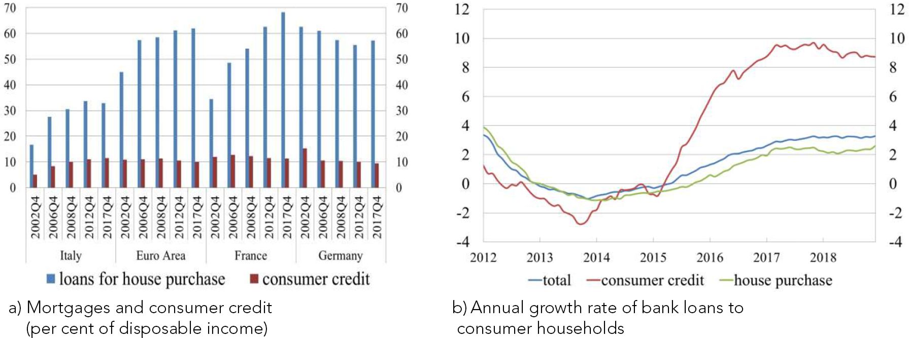
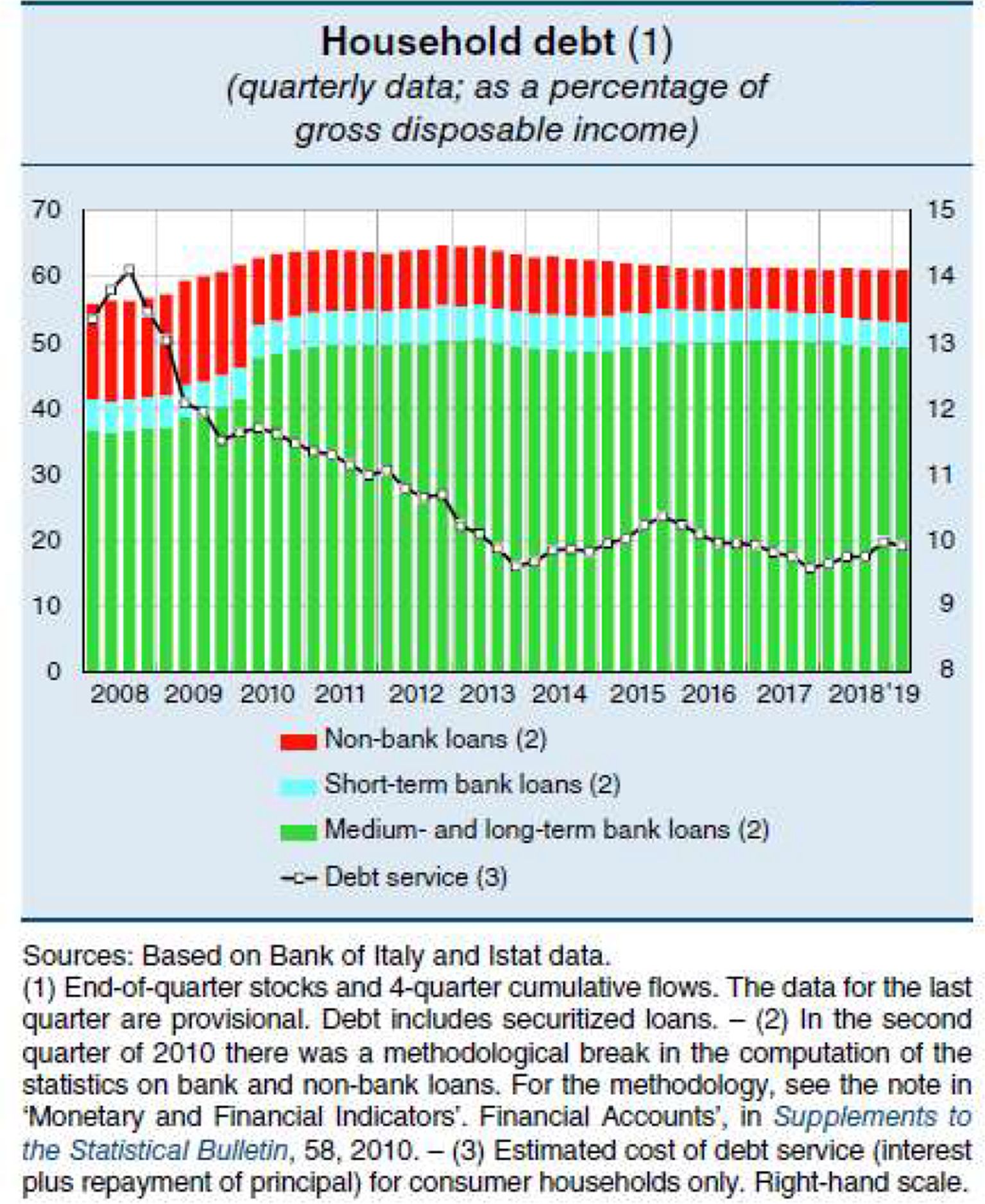
In Italy, the financial stability risks stemming from households’ debt are limited. Italian households are less indebted than European ones, though their debt-to-disposable income ratio has grown significantly since the beginning of the last decade, reaching 61.3 per cent in 2017 (37.2 per cent in 2002).1 While mortgage indebtedness has remained quite low by international standards (Figure 1a), consumer credit has strongly expanded in recent years (from −1.0 per cent in 2013 to 9.0 per cent in 2018; Figure 1b) and, as a share of disposable income, it has become very similar to that of other countries in the euro area (Magri et al., 2019).

Mortgages and consumer credit (percentages). a) Mortgages and consumer credit (per cent of disposable income), b) Annual growth rate of bank loans to consumer household.
Notes: a) Source: National accounts. b) Source: Supervisory reports
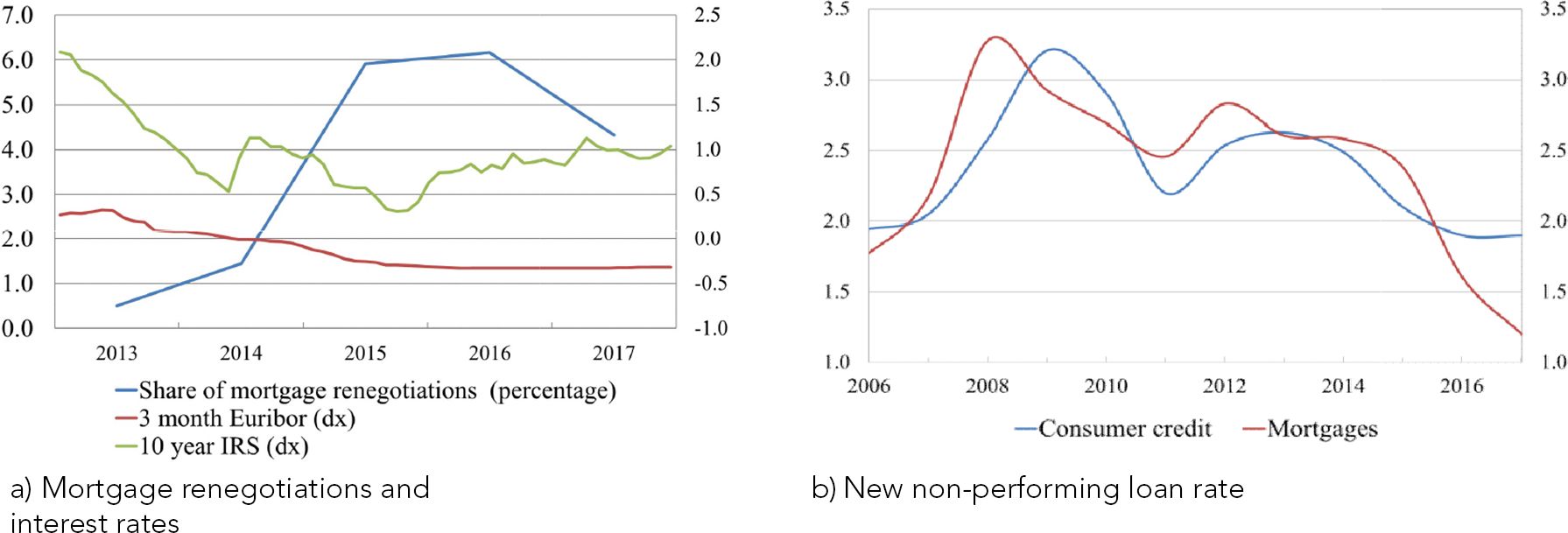
Despite the significant expansion in loans to households, the debt-service to income ratio (DSR) has not risen much and has remained at around 10 per cent (Figure A.1 in the Appendix A). In fact, the impact of higher debt on loan instalments has been mitigated in recent years by exceptionally low interest rates. Households have benefited from low rates also by renegotiating the terms of their mortgages, particularly in 2015 and 2016 (Figure 2a). Low rates and renegotiations have contributed to improving debt sustainability. The higher selectivity of banks in granting loans with respect to the pre-crisis levels has also contributed to the decrease in the new non-performing loan ratio, which has fallen from the peak of 2009 both for mortgages and for consumer loans (Figure 2b).

Mortgage renegotiations and risks (percentages). a) Mortgage renegotiations and interest rates. b) New non-performing loan rate.
Notes: a) The share of mortgage renegotiations is given by the sum of the total amount of the mortgages whose contract terms have been revised over the previous period stock of mortgages. dx means right-hand scale. Source: Supervisory reports and MIR data. b) Source: Supervisory reports for mortgages and CRIF data for consumer credit.
This evidence suggests that a timely monitoring of the risks associated with the household sector requires a model that projects the evolution of financially vulnerable households, accounting for both the dynamics of consumer credit and the possibility of revising the contract terms through mortgage renegotiation.
Several indicators of financial vulnerability have been proposed in the related literature (eg, D’Alessio and Iezzi, 2013). A first indicator that has been greatly employed by central banks to assess households’ ability to meet their debt obligations is the debt service-to-income ratio (Bank of Canada, 2011; Bank of England, 2014; Bank of Italy, 2011; European Central Bank, 2004, among others). Some studies have been carried out to assess how debt delinquency varies for different threshold values (May and Tudela, 2005; Tiongson et al., 2009; Dey et al., 2008; Beer and Schurz, 2007; Karasulu, 2008). Vacca et al. (2013) confirmed that the risk of arrears increases at a 30 per cent threshold and for households whose income net of debt payments is below the relative poverty line. A second indicator that has been used to identify financial vulnerable households is the financial margin, defined as the net income available to households after debt payments and basic living expenses (Martin and Persson, 2006; Vatne, 2006; Zajączkowski and Żochowski, 2007; Albacete and Fessler, 2010; Ampudia et al., 2016; Bettocchi et al., 2018, among others). Michelangeli and Rampazzi (2016) show that the shares of households classified as vulnerable according to both indicators (the first based on the debt service-to-income ratio and the second based on the financial margin) are similar. However, the first indicator is much simpler to compute and does not suffer from arbitrariness in the definition of some of its components, such as basic living costs. Following Vacca et al. (2013) and Michelangeli and Rampazzi (2016), we define a household as vulnerable if its debt service-to-income ratio exceeds 30 per cent and its income is below the median of the population.
To account for consumer credit growth and for the possibility of renegotiating a mortgage, which could affect the debt service-to-income ratio, we propose an extension of the microsimulation model developed by Michelangeli and Pietrunti (2014). This latter model includes the dynamics of income and mortgages (without renegotiations), while the outstanding consumer credit is assumed to be constant over time (the growth rate equals zero). These assumptions were adequate overall in the early 2010s, when mortgage renegotiations were very rare and consumer credit was growing at a relatively slow pace and up from very low levels in Italy. The recent development in household loans now means we need to accurately model the evolution over time of consumer credit and mortgage renegotiations, whose combined effect on households’ vulnerability is ex-ante unknown. The growth in consumer loans may increase vulnerability because households would face a larger loan instalment; at the same time, renegotiations act in the opposite direction by reducing periodic loan repayments. Not accounting for these dynamics may lead to a bias of an unknown sign in the projection of households’ vulnerability.
Building on the information on households’ characteristics and loan types provided in the Bank of Italy’s Survey on Household Income and Wealth (SHIW), we allow the amount and the cost of consumer loans to change over time according to the higher-frequency macroeconomic data. This implies, for instance, that a rapid increase in consumer loans can be promptly taken into account in the microsimulation model. More in detail, the projection of consumer credit is achieved in three steps: estimation of household participation, forecast of the total amount of consumer credit and computation of the instalment paid by each household. While we use an empirical approach for the first two steps, we impose some structure on the third one, assuming a standard amortization scheme. For mortgage renegotiations, we introduce simple heuristics, according to which households revise their contract terms when they pay an interest rate that is significantly above current market rates. This becomes a share of households renegotiating their mortgage that is consistent with the evidence from the SHIW.
The backtest exercises, run over the periods 2012–14 and 2014–16, show that with the new features, the model is better able to replicate (out of sample) the drop in vulnerability observed in the survey data. In particular, adding the possibility of renegotiating the mortgage terms turns out to be crucial for reproducing the downward trend observed between 2012 and 2016. Second, the new model allows us to assess how a sustained growth in consumer credit would affect households’ debt sustainability. Third, more flexible stress tests can be run.2
Finally, we provide a brief analysis on how the share of vulnerable households and the debt at risk would change if we were to define all households with a DSR of above 30 per cent as vulnerable (ie, not only those with an income below the median of the population). While households with an income below the median are the ones at a higher risk of default, this broader definition is more in line with some international studies (see, for instance, Beer and Schurz, 2007; Djoudad, 2010; International Monetary Fund, 2011; Bankowska et al., 2015).
We contribute to the literature on microsimulation models that aim at evaluating the vulnerability of households. This strand of the literature exploits detailed microeconomic data to identify which type of households are more exposed to the risk of default. By combining microeconomic and macroeconomic data, these models provide updated measures of the risks for financial stability stemming from the household sector and may even contribute to forecasting or early warning indicators. The first papers on this topic were those of Martin and Persson (2006), Vatne (2006) and Zajączkowski and Żochowski (2007) for Sweden, Norway and Poland, respectively. Among recent papers evaluating households’ vulnerability under normal conditions and scenarios of stress, we find Djoudad (2010) for Canada, Albacete and Fessler (2010) and Albacete and Lindner (2013) for Austria, Galuščák et al. (2014) for the Czech Republic, Michelangeli and Pietrunti (2014) and Bettocchi et al. (2018) for Italy, and Ampudia et al. (2016) for several European countries. Like the previous works, our paper exploits survey data, which are subject to measurement error.3 To our knowledge, our paper is the first to develop a methodology for the projections of consumer credit and mortgage renegotiations. By integrating micro and macro data, we preserve heterogeneity while exploiting the higher frequency of the macro data.
Our paper also relates to the literature on consumer credit. In recent years, many central banks have begun to publish data on consumer credit aggregates to show the main trends of this kind of debt and the emerging risks (Magri et al., 2019; European Central Bank, 2017; Bank of Italy, 2018a; 2018b). Furthermore, microeconomic data from household surveys have been exploited to capture the heterogeneity in the access to consumer credit market. For instance, Magri (2002) uses the SHIW to show that participation in consumer credit is positively correlated with income; a similar result is obtained by del Río and Young (2006) who, by focusing on unsecured debt for the years 1995 and 2000, show that the increase in participation and in the amounts borrowed are explained by the growth in household income. Magri et al. (2011) use Eurostat’s EU-SILC survey for nine European countries in the period 2005–08 to highlight that, regardless of the broad heterogeneity in participation across countries, borrowers tend to have a medium-high income, which they believe could be associated with the preference of lenders for granting loans to safer borrowers. Several papers have provided evidence of the procyclicality of debt and tried to identify the drivers of both demand and supply (Kiyotaki and Moore, 1997; Nakajima and Ríos-Rull, 2014). A robust finding is that durable consumption expenditures is procyclical as well as consumer debt (Bertola et al., 2006; Iacoviello, 2008; for a review, see Claus and Claus, 2016). Our paper proposes a novel approach for replicating the dynamics of consumer credit over time, and, in particular, for capturing the heterogeneity in the groups of households that hold this type of debt.
The paper is organized as follows: Section two describes recent developments in the Italian credit market, distinguishing between consumer credit and mortgages. Section three provides a description of households’ financial vulnerability based on the SHIW. Section four presents the model of households’ financial vulnerability that includes consumer credit dynamics and mortgage renegotiations. Section five shows the backtest exercises and the results for the baseline scenario. Section six provides a robustness analysis, focusing on all households with a DSR above 30 per cent and Section seven concludes.
2. Recent developments in loans to households
2.1 Consumer credit
Consumer credit is generally defined as a personal loan taken out to purchase goods or services, such as cars or home appliances, and overall it includes a broad list of banking and other financial products.4 In comparison with mortgages, consumer loans usually come with a higher interest rate and a shorter redemption period.
According to supervisory reports, in 2017, about 22 per cent of Italian household loans granted by banks and other financial intermediaries consisted of consumer credit (Table 1; see also Bank of Italy, 2018a). In terms of stocks, the shares of consumer credit on households’ total credit and non-performing loans (NPLs) are not negligible. In 2017, the amount of NPLs was equal to €7,035 million, much lower than the 2012 peak of €12,140 million, but this was still a high share of total NPLs (14.2 per cent).
Loans to households (millions of euros and per cent)
| Mortgages | Consumer credit | Total loans | Percentage composition | |||||||
|---|---|---|---|---|---|---|---|---|---|---|
| Total | Non-performing | Total | Non-performing | Total | Non-performing | A/E | B/F | C/E | D/F | |
| (A) | (B) | (C) | (D) | (E) | (F) | |||||
| 2010 | 329,950 | 13,938 | 118,779 | 10,766 | 543,902 | 38,765 | 60.7 | 36 | 21.8 | 27.8 |
| 2011 | 345,406 | 16,055 | 118,476 | 11,792 | 565,345 | 46,760 | 61.1 | 34.3 | 21 | 25.2 |
| 2012 | 345,255 | 18,845 | 116,142 | 12,140 | 562,102 | 52,173 | 61.4 | 36.1 | 20.7 | 23.3 |
| 2013 | 341,952 | 21,728 | 111,937 | 12,088 | 554,170 | 57,161 | 61.7 | 38 | 20.2 | 21.1 |
| 2014 | 341,221 | 23,660 | 108,644 | 10,879 | 549,522 | 59,087 | 62.1 | 40 | 19.8 | 18.4 |
| 2015 | 342,698 | 25,530 | 109,993 | 9,632 | 551,824 | 60,922 | 62.1 | 41.9 | 19.9 | 15.8 |
| 2016 | 348,643 | 25,812 | 113,302 | 7,804 | 558,341 | 57,592 | 62.4 | 44.8 | 20.3 | 13.6 |
| 2017 | 355,906 | 23,588 | 121,992 | 7,035 | 567,262 | 49,521 | 62.7 | 47.6 | 21.5 | 14.2 |
| 2018-Q3 | 356,792 | 20,295 | 129,257 | 6,618 | 571,742 | 40,233 | 62.4 | 50.4 | 22.6 | 16.4 |
-
Source = Supervisory reports.
2.2 Mortgages
A mortgage is a loan in which a real estate property is used as collateral. In a residential mortgage market, the borrower pledges its house to the lender (typically a bank), which has a claim on the house if the borrower is unable to meet their debt obligations. Mortgages are the main liability of the household sector and they accounted for about 63 per cent of total Italian household loans in 2017 (Table 1).
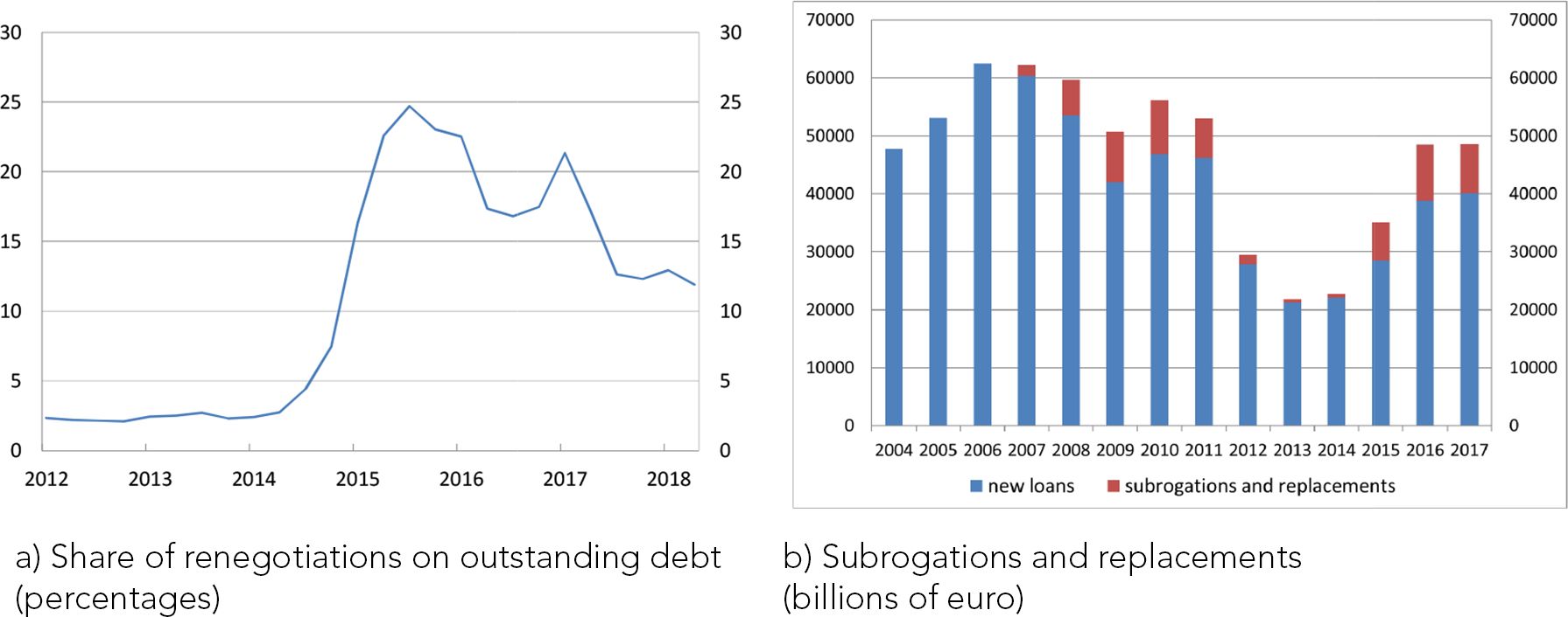
In recent years, in face of the very low market rates and of the possibility of changing the mortgage terms offered by the introduction of the ‘Bersani Decree’, mortgage renegotiations have gained importance. We can distinguish between three different types of mortgage renegotiations: renegotiation with the same bank (variations in some mortgage characteristics, such as duration, rate type, but not amount, with the same bank), subrogation (portability, shift of the mortgage from one bank to another), and replacement (mortgage cancellation and formalization of a new loan with the same or a different bank).5 These three types have in common that, after refinancing, households normally reduce their debt service, thereby also decreasing their probability of default. As shown in Figure 3, from 2015 onwards, in a period of very low interest rates, these three types of mortgage refinancing have become more frequent than in the previous three years.

Mortgage refinancing. a) Share of renegotiations on outstanding debt (percentages), b) Subrogations and replacements (billions of euro).
Notes: Our calculation based on Supervisory reports.
3. SHIW data
3.1 Descriptive statistics
Our analysis exploits the 2010–16 waves of the SHIW, a survey that comprises about 8,000 households distributed over roughly 300 Italian municipalities.6 In each wave of the survey, half of the sample is longitudinal and half is renewed (unbalanced panel). The dataset contains information on household demographic characteristics (age, education, family composition and so on) as well as consumption, income, wealth and liabilities. With respect to the latter item, households are asked to distinguish between mortgages on their first house or on other real estate, and consumer credit. Loans for household needs other than property purchase or renovation represent the main part of consumer credit (around 80 per cent) whereas bank overdrafts and credit card receivables only account for 16 and 4 per cent respectively.7 For loans other than bank overdrafts and credit card receivables, households declare the outstanding debt amount, the initial amount borrowed, the year when the loan was originated, its maturity, the annual instalment, the interest rate paid and the rate type (adjustable rate or fixed rate). In 2014 and 2016, questions aimed at capturing the mortgage renegotiations were also introduced.
Summary statistics on vulnerable households are based on the pooling of the four cross-sections (31,679 observations). The estimation of the models presented in Section four is based on the longitudinal component of SHIW, where we keep households who stay in the sample for at least two waves (17,368 observations). The baseline simulation exercise presented in Section 5.2 is based on the last wave of SHIW (7,421 observations).
3.2 Household vulnerability
Vulnerable households are those with a DSR above 30 per cent and income below the median of the population. Their identification implies the computation of the DSR for each household, as it is not directly contained in the survey. To this end, we exploit the information provided by the household on instalments for mortgages and for loans for needs other than property purchase or renovation. This information is not available for credit card receivables and bank overdrafts,; we thus assume that each year the whole credit card debt and one fifth of bank overdrafts are repaid. The assumption on the repayment of credit card debt is quite natural, since it is often repaid in a few months; that on bank overdrafts comes from the fact that in Italy they must be repaid upon the bank’s request, but usually this type of debt is not repaid for several years. We therefore assume that a household repays the total bank overdraft in five years, which is on the one hand, a credible amount of time if we look at the dynamics of bank overdrafts within the longitudinal component of the SHIW, but on the other hand it is also a conservative choice (meaning that it tends to amplify debt-service ratios), since bank overdrafts could be repaid in more than five years.
According to the SHIW data, the share of vulnerable households in the period 2010–16 was around 2 per cent, with a peak of 2.9 per cent in 2012, which then decreased to 1.6 in the last wave. The debt at risk was around 16 per cent in the same period, going from 19.0 per cent in 2012–10.4 per cent in 2016.8
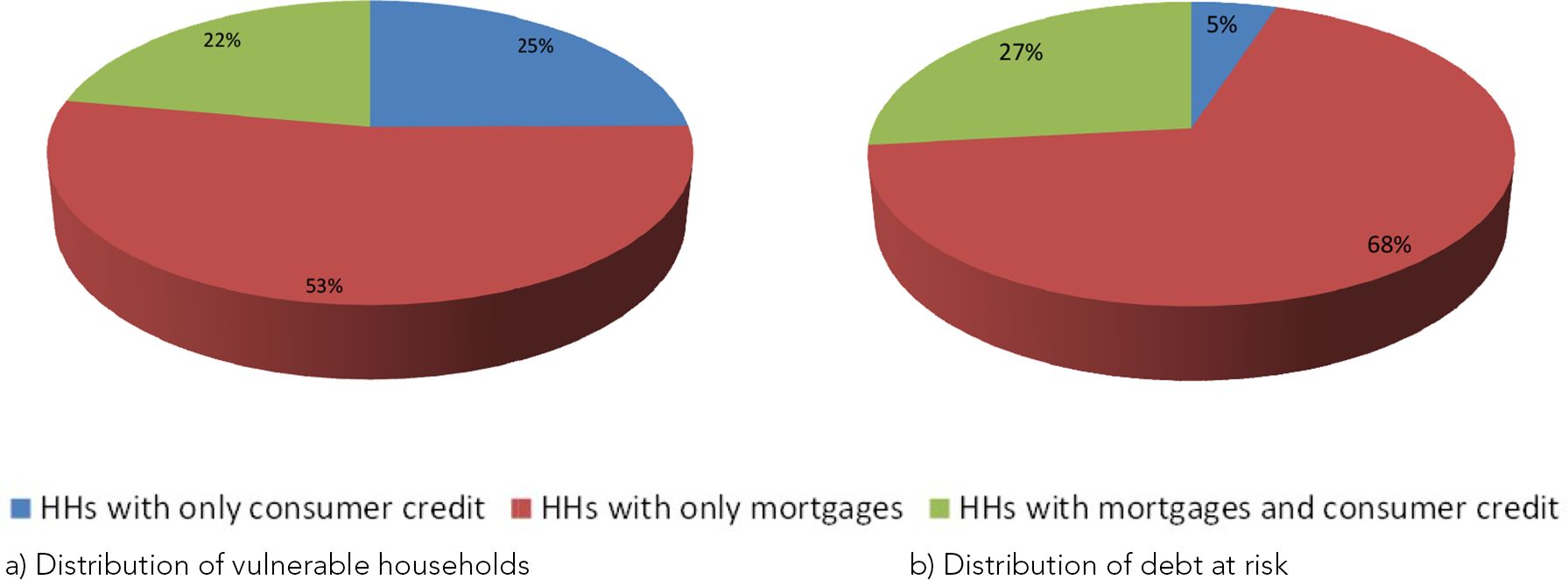
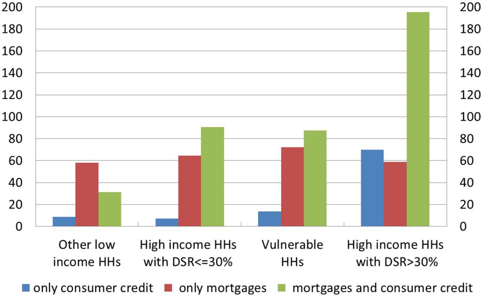
A closer look at vulnerable households indicates that almost 50 per cent of them have consumer credit, often together with a mortgage (Figure 4a), and hold over 30 per cent of the total debt at risk (Figure 4b). The share of debt at risk held by those with only consumer credit (without a mortgage) is, however, much lower (5 per cent).

Financial vulnerability by type of debt (averages 2010–16; percentages). a) Distribution of vulnerable households, b) Distribution of debt at risk.
Notes: Our calculation based on SHIW data. Debt at risk refers to the debt held by vulnerable households.
The average amount of consumer credit held by vulnerable households (€10,000; Table 2) is significantly lower than that associated with mortgages (about €80,000). This suggests that the risks for financial stability due to consumer credit in isolation are low overall, but they are not negligible if consumer credit is combined with mortgage debt. With respect to other low-income households, vulnerable households are charged higher interest rates on both mortgages and consumer credit; these higher rates can reflect the higher riskiness perceived by the banks but, at the same time, could diminish the households’ ability to repay their debt.
Household debt (averages 2010-16; euros and per cent)
| Consumer credit | Mortgage | |||
|---|---|---|---|---|
| Amount | Interest rate* | Amount | Interest rate* | |
| Vulnerable HHs | 10,001 | 5.0 | 80,734 | 4.3 |
| Other low-income HHs | 5,446 | 4.4 | 52,009 | 4.1 |
-
Notes: Our calculation based on SHIW data.
-
*
Interest rates are calculated as weighted averages of the amount borrowed. Other low-income households include households with an income below the median of the population and a DSR below 30 per cent.
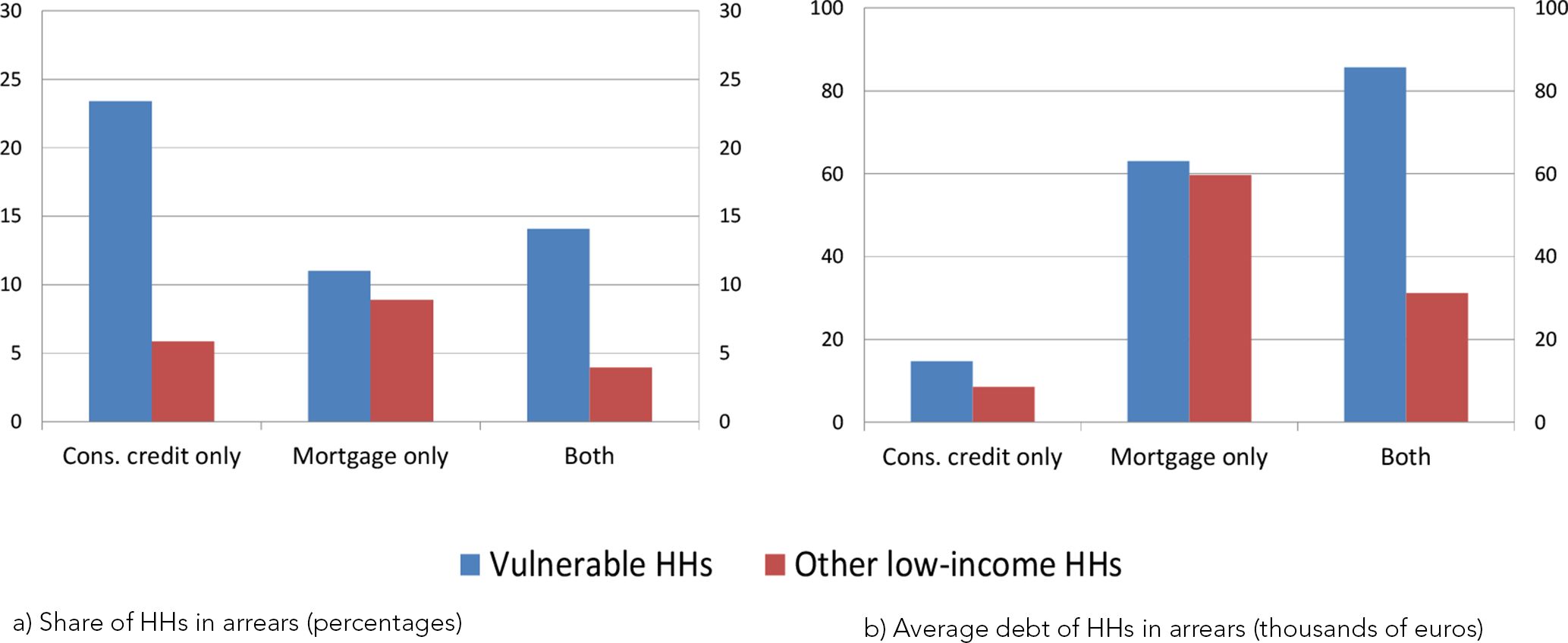
To further assess the financial fragility of vulnerable households, we look at those that declare themselves to be in arrears by more than 90 days. Being in arrears does not necessarily imply defaulting, but it is reasonable to assume that households in arrears are at a higher risk of experiencing debt sustainability issues. As expected, vulnerable households are more likely to be in arrears and when they are, they have higher debts than other low-income but non-vulnerable households (Figure 5). More specifically, 23 per cent of vulnerable households with only consumer credit are in arrears, compared with about 6 per cent for the other low-income non-vulnerable ones. The figure also indicates that households tend to be in arrears more often when debt is represented by consumer loans rather than mortgages.

Financial vulnerability and arrears of more than 90 days (averages 2010-16). a) Share of HHs in arrears (percentages), b) Average debt of HHs in arrears (thousands of euros).
Notes: Our calculation based on SHIW data. Other low-income households include households with an income below the median of the population and a DSR below 30 per cent.
Another indicator of debt sustainability is a household’s subjective perception of economic difficulty, measured by the share of households that declare that their income is not sufficient to see them through to the end of the month without difficulty. The share of households that face financial difficulties is higher among vulnerable households than among other low-income ones (Figure 6). Furthermore, this share is particularly pronounced among households that only have consumer credit, while those that also have a mortgage declare a much better perception of their economic situation.
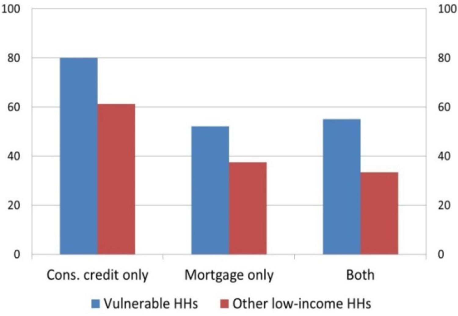
Subjective perception of economic difficulty (1) (percentages; averages 2010–16).
Notes: Our calculation based on SHIW data. (1) Share of households declaring that their income is not sufficient to see them through to the end of the month without difficulty.
With exceptionally low rates, mortgage renegotiations have likely contributed to mitigating households’ difficulties in meeting their debt payments in recent years. However, survey data on mortgage renegotiations are limited and only a few simple statistics can be reliably calculated.9 According to the SHIW data, about 8 per cent of indebted households revised their contract terms (5 per cent in 2014, 12 per cent in 2016) and around 30 per cent of them had both mortgages and consumer credit. Households that chose to revise their mortgage terms were, on average, paying higher interest rates than other households in the previous wave; after renegotiation, the rate charged was lower. About one third of these households moved from a condition of vulnerability to one of non-vulnerability.
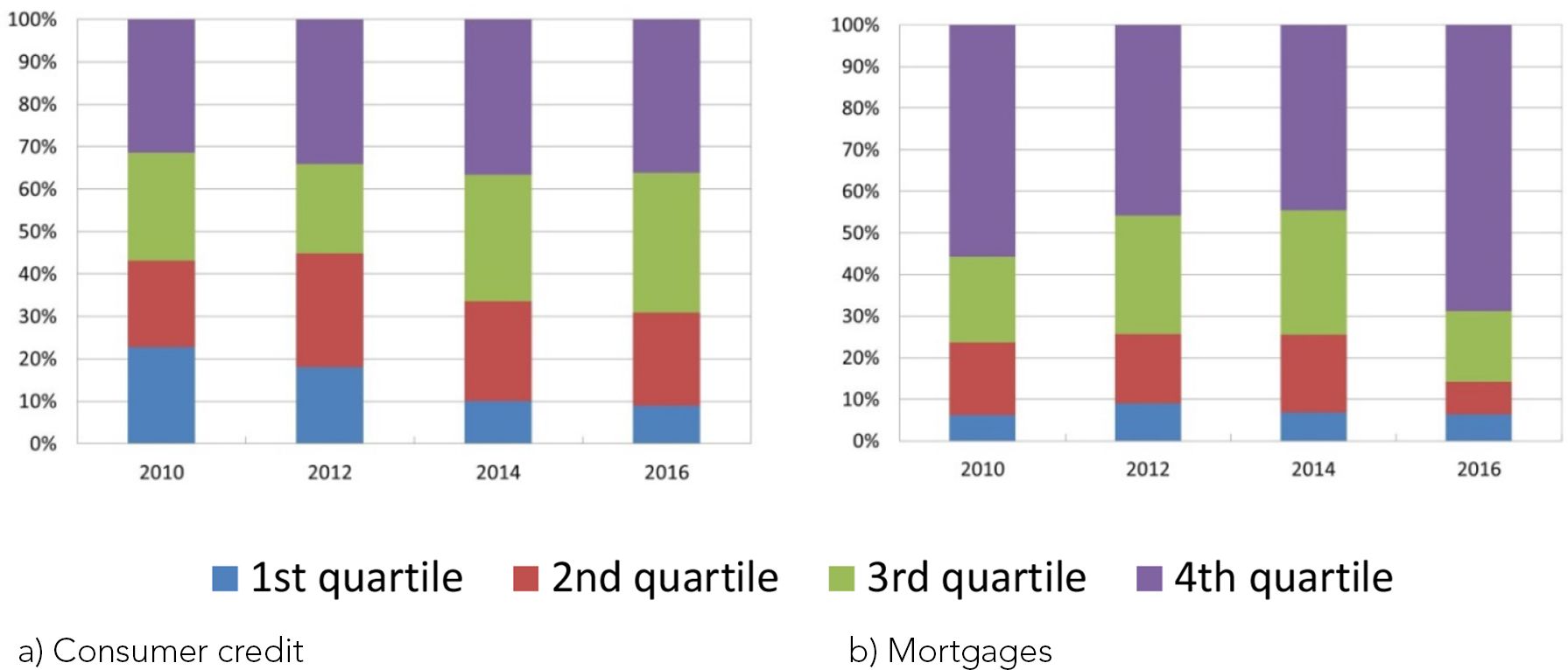
Finally, bank selectivity in granting loans coupled with households’ choices have driven changes in the distribution of debt across income quartiles. In 2010, consumer loans were quite uniformly distributed across household income groups (Figure 7). This implied that low-income households were proportionally bearing a much higher consumer debt than high-income ones. Instead, in 2016, the vast majority of mortgages were concentrated among households with an income above the median of the population and similarly, the share of consumer credit held by high-income households has progressively increased. This suggests that the ability of the household sector to sustain debt payments has been on the rise.

Household debt by income groups. a) Consumer credit, b) Mortgages.
Notes: Our calculation on SHIW data.
4. Modelling households’ vulnerability including consumer credit and mortgage renegotiations
In this section, we describe how we built our projections of households’ vulnerability over time. Specifically, we present the approach employed to model both consumer credit dynamics and mortgage renegotiations.10 For the projections of income and mortgage instalments, we rely on the modelling approach described in Michelangeli and Pietrunti (2014).11
With respect to consumer credit, we took a three-step approach. First, we modelled households’ participation in the consumer credit market; second, we projected households’ loan amounts, replicating the macro growth rate of consumer credit; and finally, we computed the instalments using a standard French amortization schedule. For mortgage renegotiations, we assume that households revise their contract terms if their mortgage rate is significantly above current market rates.
4.1 Modelling consumer credit
4.1.1 Participation in the consumer credit market
For each household i, participation in the consumer credit market in period t depends on participation in the previous period in both the consumer credit market and in the real estate market, on the income quartile, and on the purchases of consumer durables:
where is a dummy variable equal to one if household i has a consumer loan in year t and zero otherwise, is a dummy variable equal to one if household i has a mortgage loan in the previous period and zero otherwise.12 is a vector of income quartile dummies. is a vector of household durable consumption dummies. We prefer to use a vector of dummies for the amount of durable consumption, rather than a continuous variable, to minimize the errors associated with the projections of this variable. We consider five intervals, which were chosen starting from its sample distribution. We thus have five different dummy variables, , each of which takes the value 1 if the continuous consumption falls in the respective interval and zero otherwise.13 We assume that the errors are normally distributed.
The regression was estimated using a linear regression model.14 The regression coefficients imply that households with higher income and belonging to the higher classes of durable consumption are more likely to have a consumer loan. Furthermore, having a consumer debt or a mortgage in the previous period is associated with a higher probability of participating in the consumer credit market in the current period (Table A.1). The process is thus characterized by high persistency, which could be due to true state dependence or to individual-specific permanent unobserved heterogeneity. For instance, an individual may participate in the consumer credit market because of some unobserved characteristics, such as the need for money, despite other observed characteristics. In our approach, we set all individual effects equal to zero. Richiardi and Poggi (2014) show that this approach is optimal when the goal is forecasting mean values and the model is linear.15
The coefficients for each regressor , as well as the mean and the standard deviation of the error term, were then used to simulate each household’s participation in the consumer credit market. We ran 50 different simulations to have some variability in the estimated error term.16
The estimated probability of entering the consumer credit market for each household in each period is given by:
In our setup, always takes values of between zero and 1. However, for simulation purposes, we are not interested in a continuous probability, but in identifying which households participate in the consumer credit market and which households do not. In other words, we need a variable equal to one for participants and equal to zero for non-participants. Thus, for each year, we first ordered our households based on their probability of participation ,, from the highest to the lowest. Then, we selected a threshold , above which all households are assigned for participating in the consumer credit market. The threshold is chosen to capture recent trends in participation.17
The simulated value of the participation in the consumer credit market for household i is:
4.1.2 Projection of the consumer loan amount
After having established whether a household participates in the consumer credit market, we needed to assign a value for the consumer loan amount. We assumed that changes in consumer credit depend on household income quartile, on household consumption of durables, and on the aggregate dynamics of consumer credit.
Therefore, for each household i that had already participated in the consumer credit market in the previous period, we computed the change in the consumer credit amount
and then we ran the following regression:
where is the growth rate of consumer loans to households in the Italian economy.
The results of equation (4) are reported in Table (A.2) in Appendix A. As expected, has a positive sign, reflecting the fact that a stronger aggregate credit growth translates into higher average household consumer credit. Households with higher consumer durable expenses, ie, those belonging to the fifth class, tend to have larger positive changes in consumer credit.
For each household i already participating in the consumer credit market, the estimated change in consumer credit at time t is computed using the coefficient of the regression (4):
The projection of the consumer loan amount over time is given by the previous period loan amount plus the estimated change:
For the first period of the simulation, we have actual data on from the SHIW; in the following periods, is derived from the model.
For households that are estimated to have participated in the consumer credit market at time (t+1) for the first time, we do not have the previous period’s consumer credit, thus we estimated the loan amount by means of a pseudo-panel. First, we created G groups of similar households based on their age class, job type, durable consumption class, and mortgage tenure. Second, we estimated equation (4) for the median group change in the consumer loan amount, . Third, a household i, that belongs to group g and enters the consumer credit market at time t, was assigned the loan amount estimated on the pseudo-panel regression:
After having computed the loan amount for each household that participates in the consumer credit market, we constructed the total consumer debt in the simulated economy:
Then, we calculated the growth rate of the consumer credit loan in our simulation and we compared it with the actual aggregated data. As our goal was to have similar growth rates, we introduced a multiplicative adjustment factor for each household loan amount, which then became equal to . For instance, in the 2016–18 simulation, it equals 1.08 for the first year and 1.09 for the second year. These adjustment factors are not high and appear reasonable, especially if we account for the fact that the survey data could have problems of misreporting and that households are not selected to be representative with respect to their consumer credit debt.
4.1.3 Annuitization of consumer loans
Once we have the projected consumer debt we can perform an annuitization to calculate (annual) instalments. Assuming that consumer debt is repaid by a French amortization schedule, we need to make assumptions on maturity and interest rates.
For households having already consumer debt in the survey data, we use the maturity and interest rates available in the survey. For the households having more than one personal loan, we calculate an average maturity and an average interest rate, and we aggregate all debts in a single one (only loans for household needs other than property purchase, credit card receivables, and bank overdrafts are considered).
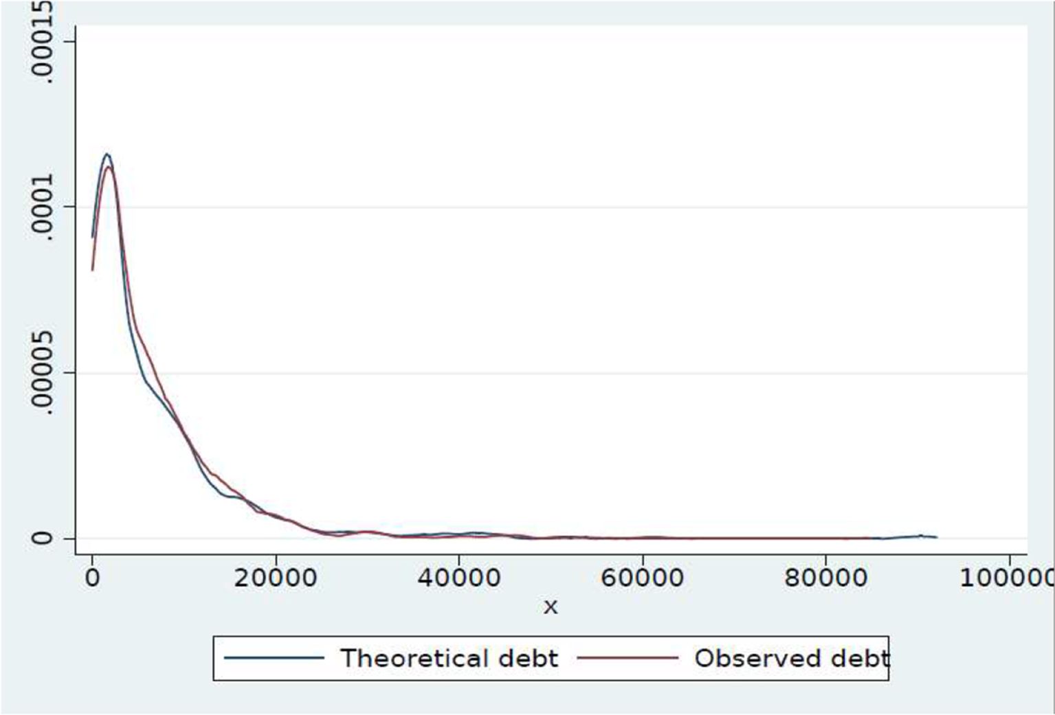
The theoretical debt that would be consistent with the observed instalments, under the assumptions just mentioned (remember that in t=0 we observe both instalments and debt), is very close to the actual declared debt (Figure 8).

Distribution of theoretical and observed debt (1).
Notes: Our calculation based on SHIW data. (1) Observed debt refers to the actual SHIW outstanding debt for each household. Theoretical debt refers to the amount of debt that would be consistent with the installments paid by each household.
Depending on whether the change in consumer credit () is negative or positive we have two different approaches. In the first case, , we assume (partial) reimbursement of the outstanding debt. In the second case, , we assume that a new contract of consumer credit is signed, and its instalments are added to those of the old (already outstanding) debt. The new loan has the same maturity as the old one at origination and the same type of interest rate (fixed vs variable). We therefore assume that a household’s preferences for maturity and type of interest rate remain constant over time.
For those that do not already have consumer debt at t=0, but are projected to participate in the consumer credit market in the following years, we assume that they choose a variable interest rate, sign their contract at the current rate, and, based on the observed data, set the debt maturity at 5 years.18
4.2 Modelling mortgage dynamics with renegotiations
Supervisory reports indicate that mortgage renegotiations have gained importance in recent years. We extend the model by Michelangeli and Pietrunti (2014) to allow for the possibility of households revising their mortgage terms.
Since only a few households in the SHIW declare they have renegotiated their debt, we cannot develop an extension of the model that exploits a household’s characteristics. Our novel modelling approach therefore relies on a few assumptions that are necessary to capture the heterogeneity of mortgage renegotiations. We assume that mortgage renegotiation occurs when households pay a mortgage rate that is at least 3 percentage points higher than the reference rate plus a household’s specific spread. After renegotiation, the bank sets a rate equal to the current reference rate plus the household’s spread.
More in detail, we exploit the SHIW information on the mortgage rate declared to be paid by household i at time t, and we assign to each household a reference rate which depends on its loan characteristics (year of origination and rate type).19 Then, for indebted households we calculate the mortgage spread, , starting from the standard relationship:
For fixed-rate mortgages, the spread is calculated as the difference between the mortgage rate declared to have been paid at time t and the 10-year euro interest rate swap (IRS) at origination; for variable-rate mortgages, the spread is given by the difference between the declared rate in year t and the 3-month Euribor in the same year. The spread reflects the differences in households’ riskiness and it is highly heterogeneous across households. Regression coefficients imply that the spread is higher for households with low education levels, for those living in the South, and for those that are self-employed or not working (Table A.3). When the household’s spread turns out to be negative, likely due to mistakes in answering the survey’s questions, we assign the median spread of the group of households with similar characteristics (education, geographic area and occupation).
We assume that at time t a household renegotiates its debt if its mortgage rate exceeds the sum of current period reference rate , its specific spread, and a parameter : 20
is set as equal to 3 percentage points. This parameter’s value has been selected as it allows us to obtain model statistics on the share of households that renegotiate their mortgage terms (Table 3, Panel a) and on the share of debt that they hold (Table 3, Panel b) that are reasonably close to those based on the SHIW data.21
Mortgage renegotiations (percentages)
| SHIW | MODEL* | |
|---|---|---|
| a) Share of households that renegotiate their mortgage terms among indebted households | ||
| 2014 | 5.0 | 5.4 |
| 2016 | 11.7 | 12.6 |
| b) Share of debt held by households that renegotiate their mortgage terms | ||
| 2014 | 4.0 | 2.8 |
| 2016 | 14.9 | 12.0 |
-
*
Averages over two years.
We assume that banks do not modify the spread applied to each household, ie, if a household was considered risky when the mortgage was initially granted, the household would continue to be so and the bank would charge the same spread.22 Upon renegotiation, the new mortgage rate faced by the household equals the current period reference rate plus the household’s spread:
5. Model results
In this section, we present the results obtained by simulating the model under different specifications. We define the model described in Michelangeli and Pietrunti (2014) as ‘old’ and the model augmented with both mortgage renegotiations and consumer credit dynamics as ‘new’. The macroeconomic inputs to the model are described in Appendix B.
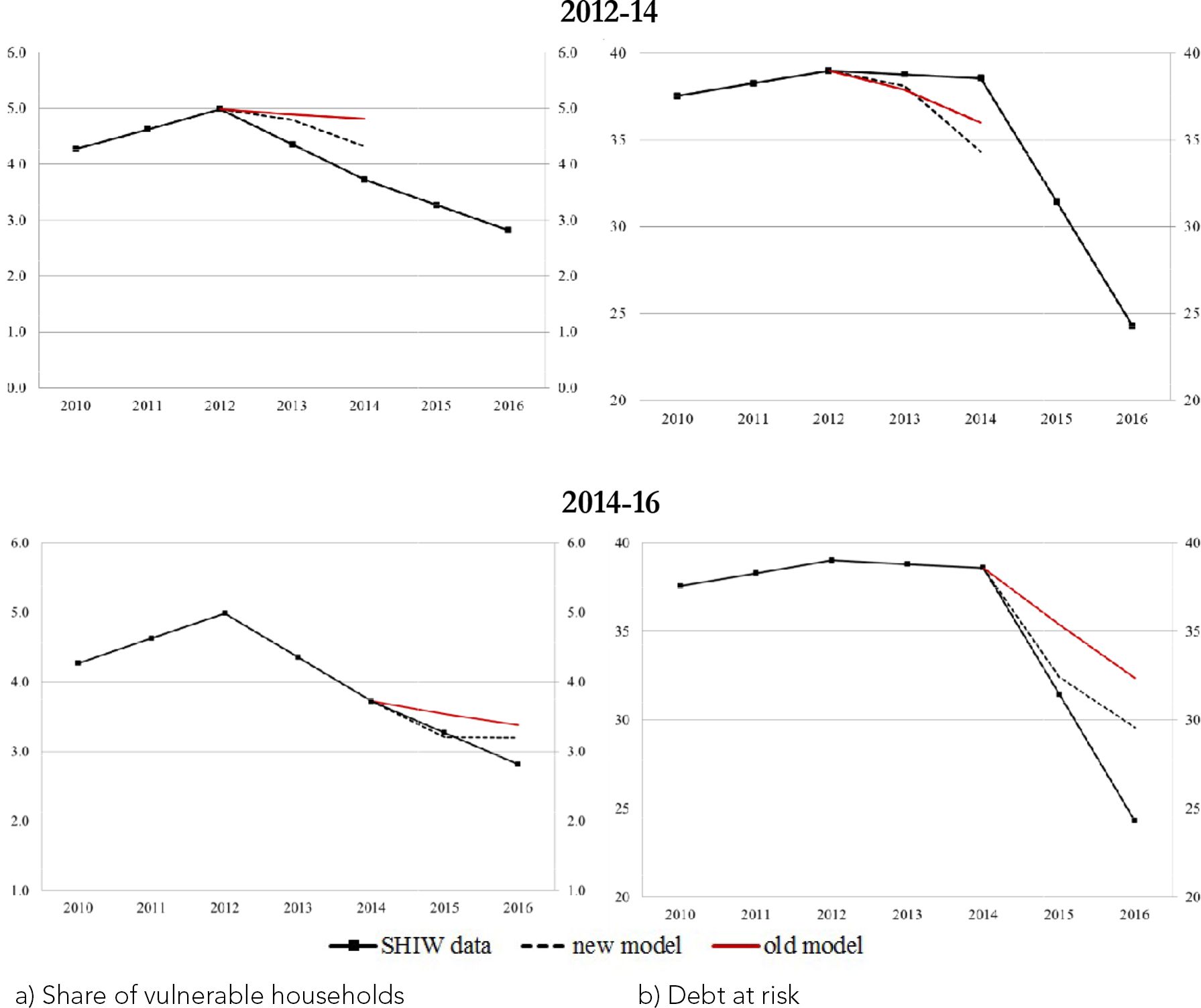
5.1 Backtesting
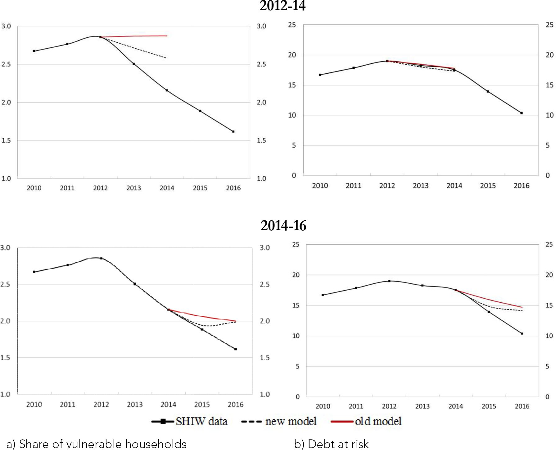
To evaluate the model’s performance in terms of the accuracy of its projections, we carried out backtest exercises on two waves of the SHIW. Starting from either the 2012 or the 2014 wave, we present here the two-year out-of-sample predictions of the share of vulnerable households in the population and the share of total debt held by them (Figure 9).

Backtest exercises – Vulnerability (percentages). a) Share of vulnerable households, b) Debt at risk.
Notes: Debt at risk refers to the share of debt held by vulnerable households. The black line with diamonds represents actual SHIW data; the red and the dotted lines represent the out-of-sample projections for the ‘old model’ and the ‘new model’ respectively. These projections correspond to the median values across 50 simulations for the two model specifications.
For the period 2012–14, characterized by positive economic growth, the low interest rates and the contraction in consumer credit contributed to the reduction in the share of vulnerable households. Instead, with respect to the debt at risk, the differences between the two models are negligible reflecting the fact that a contraction in the share of vulnerable households with consumer credit has a limited impact on the total debt at risk. For the period 2014–16, in a context of very low interest rates, accounting for the possibility of revising the contract terms through renegotiations is crucial for a better prediction of both indicators of vulnerability.
Overall, both backtesting exercises show that the ‘new model’ has superior out-of-sample predictions overall and is better equipped to capture the downward trend of vulnerability observed in the last few years.
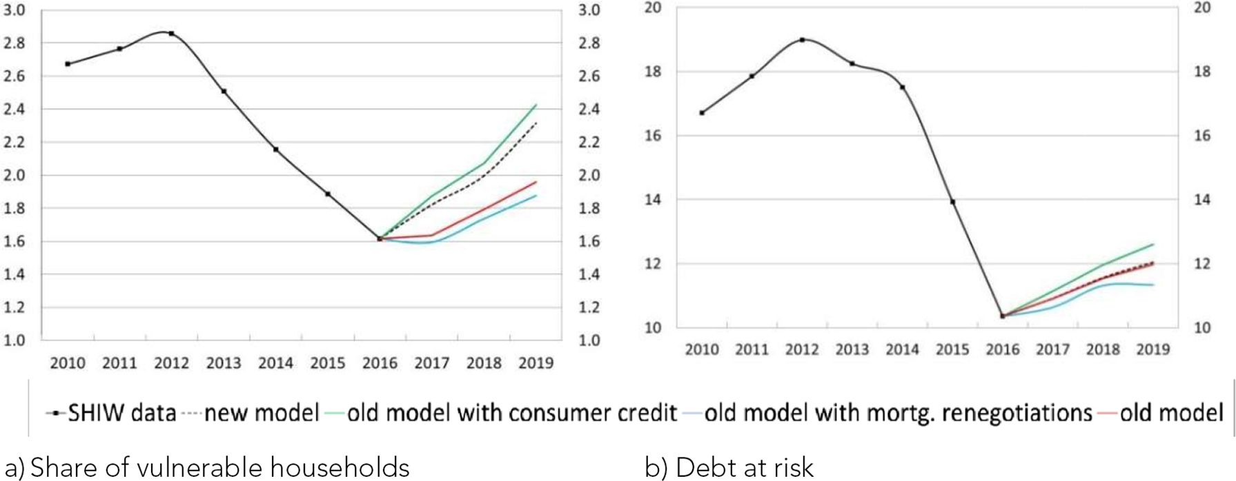
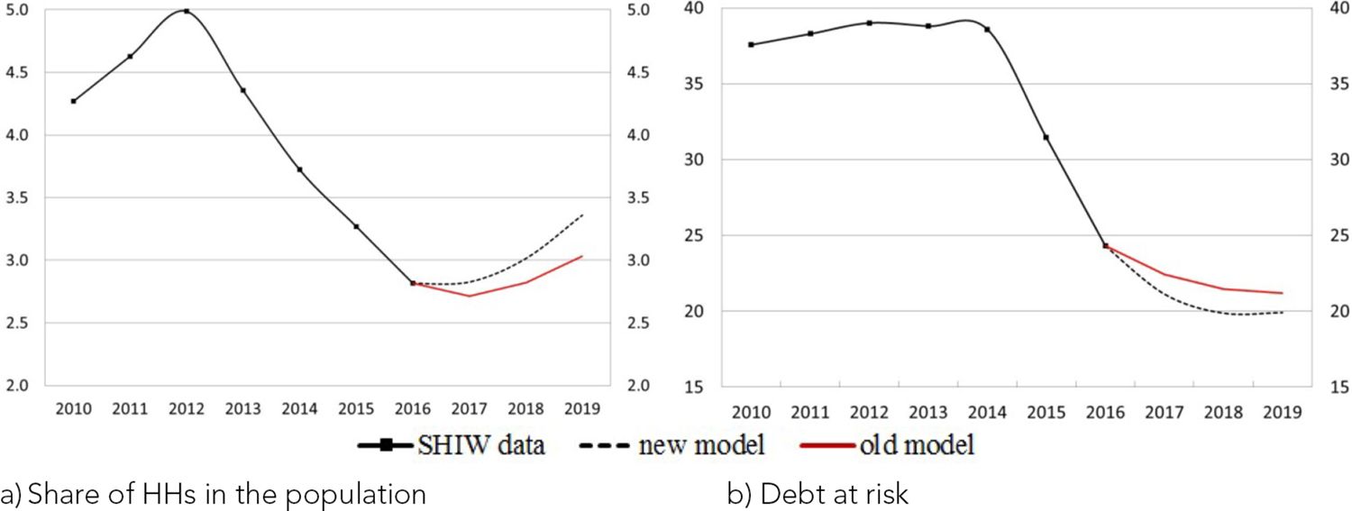
5.2 Baseline simulation over the period 2016-19
Figure 10 shows the prediction of the share of vulnerable households (Panel a) and the share of total debt held by these households (Panel b) in 2019 starting from 2016, the most recent SHIW wave. According to all model specifications, household vulnerability is projected to increase. The ‘new model’ indicates that between 2016 and 2019, the percentage of vulnerable households may have increased from 1.6 to 2.3 per cent, while the share of debt at risk may have only changed slightly, from 10.4 to 12.0 per cent.23

Vulnerability in the period 2016-2019 (percentages). a) Share of vulnerable households, b) Debt at risk.
Notes: Debt at risk refers to the share of debt held by vulnerable households.
In the first year of the simulation, the projections of the ‘old model’ indicate that the share of vulnerable households remained essentially stable as the increase in income growth, coupled with the low interest rate, was sufficient to compensate for the effects of the increase in the growth rate of mortgages. The ‘new model instead projects an increase in the share of vulnerable households, which is entirely driven by the high growth rate of consumer credit. In the second year of the simulation, a rise in interest rates, which affects both the loan payments of households holding a variable interest rate mortgage and those associated with new originations, and a positive credit growth (for both mortgages and consumer credit) contributed to the increase in the share of vulnerable households despite a positive income growth. The total effect is more pronounced in the ‘new model’, when consumer credit growth is also considered. In the last year of the simulation, 2019, higher interest rates and growth rate of consumer credit are expected to drive a further increase in the percentage of vulnerable households.
In terms of debt at risk, the differences between the ‘old’ and the ‘new’ models are negligible, since the negative effects on vulnerability associated with the expansion of consumer credit are compensated by the positive effects associated with mortgage renegotiations.
6. Robustness exercise: Extension of the analysis to all households with a DSR above 30 per cent
We have so far focused on households with a DSR above 30 per cent and an income below the median of the population. This choice is because highly indebted low-income households are the most fragile and display the highest default risks (Vacca et al., 2013).
However, as a robustness check and in line with other studies in the related literature (Djoudad R., 2010, among others), we also monitor highly indebted households with a high income. Specifically, we analyse the risks relating to households with a DSR above 30 per cent and an income above the median of the population. As shown in Table 4, even though this group of households represents a small share of the population, it holds about 20 per cent of the total household debt. Interestingly, the share of households without any debt is very high and similar for high-income households with a DSR ≤30 per cent and for other low-income households (respectively, 82 and 88 per cent for each group).
Distribution of households by income and DSR (percentages; averages over the period 2010-16)
| Share of households | Share of debt | |
|---|---|---|
| Vulnerable HHs | 2.3 | 15.8 |
| Other low-income HHs | 47.7 | 13.9 |
| High-income HHs with DSR >30% | 1.5 | 18.3 |
| High-income HHs with DSR ≤30% | 48.5 | 52.0 |
-
Notes: Our calculation based on SHIW data. High-income households are those with an income above the median of the population.
The importance of this group for financial stability analysis is shown by the probability of being in arrears by more than 90 days, which is about 4.1 per cent, whereas it is only 1.4 per cent for high-income low-DSR households. Moreover, the former group of households in arrears is considerably more indebted than all the other groups (Figure 11).

Average amount of debt among households in arrears (thousands of euros, average over 2010-16).
Notes: Our calculation based on SHIW data. High-income households are those with an income above the median of the population.
We construct a liquidity index, equal to the ratio of liquid financial assets (deposits, certificates of deposits, repos and postal accounts) to loan instalments. This index measures the number of years during which a household could service total debt only with its liquidity. High- and low-income households with a DSR above 30 per cent have a similar liquidity index (Table 5), suggesting that all households with a DSR above 30 per cent emerge as particularly fragile since they can only cover their debt instalments for less than one year with their most liquid assets. Moreover, households with a DSR above 30 per cent are very similar also with respect to other stock indicators that are considered relevant for identifying households’ fragility, such as the debt-to-income ratio and the debt-to-assets ratio.
Indicators of indebted households (percentages; averages over the period 2010-16)
| Vulnerable HHs | Other low income HHs with DSR <30% | High income HHs with DSR >30% | High income HHs with DSR <30% | |
|---|---|---|---|---|
| Total wealth | 118416.5 | 97649.57 | 343556.8 | 364953.6 |
| Financial wealth | 4628.9 | 7228.245 | 26838.81 | 46315.7 |
| Liquid assets | 3468.2 | 5614.0 | 13404.5 | 21399.0 |
| Liquidity index (fa/instalment) | 0.795 | 6.440 | 0.828 | 15.117 |
| Debt to income | 4.041 | 0.118 | 3.166 | 0.200 |
| Debt to assets | 1.689 | 0.024 | 1.608 | 0.011 |
-
Notes: Our calculation based on SHIW data. fa indicates liquid financial assets. High-income households are those with an income above the median of the population.
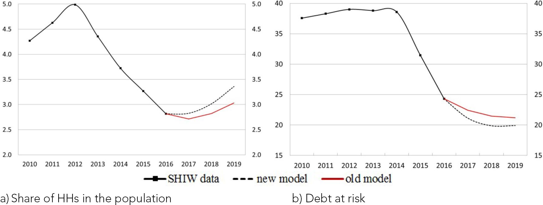
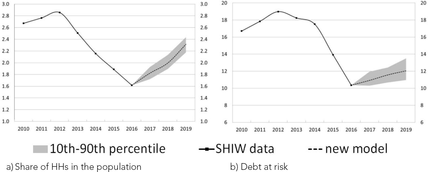
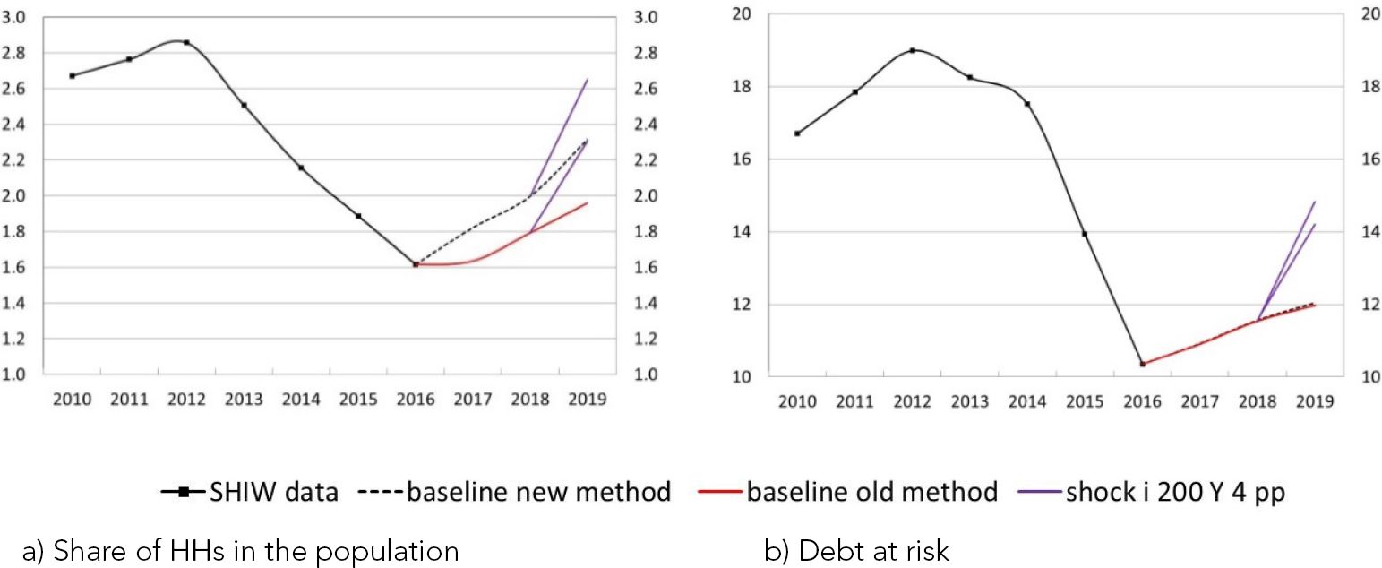
Figure 12 shows the baseline projections for the period 2016–19.24 With this broader definition, the share of vulnerable households in the population in 2016 is about 1 percentage point higher (2.8 per cent) and the share of debt at risk is about 14 percentage points higher (24.3 per cent) than in the case where only households with a DSR above 30 per cent and an income below the median are considered. According to the ‘new model’, the share of vulnerable households is projected to have increased to 3.4 in 2019, in response to the significant consumer credit growth. The share of debt held by all vulnerable households instead would fall from 24.3 to 19.9 per cent between 2016 and 2019. In this case, the reduction would be greater than that estimated only for low-income vulnerable households. This is because the effect of mortgage renegotiations is more relevant for high-income highly indebted households.
All households with DSR >30 per cent in the period 2016–2019 (percentages). a) Share of HHs in the population, b) Debt at risk.
Notes: Debt at risk refers to the share of debt held by households with DSR above 30 per cent.
7. Conclusion
This paper presents a novel modelling approach for the evolution of consumer credit and mortgage renegotiations within a microsimulation model of households’ vulnerability. In particular, an extension of the model by Michelangeli and Pietrunti (2014) is provided to account for the recent increase in consumer credit and its progressive concentration among the high-income households, and to account for the wide recourse to mortgage renegotiations occurring in a context of very low interest rates.
These new features of the microsimulation model have proved to be crucial for carefully assessing the financial stability risks stemming from the household sector. The model with consumer credit and mortgage renegotiations outperforms Michelangeli and Pietrunti (2014) in capturing the trends of vulnerability over the last few years.
Both mortgage renegotiations and consumer credit affect vulnerability, though in opposite directions. By reducing loan instalments, mortgage renegotiations contribute to decreasing vulnerability. Consumer credit instead drives an increase in the share of vulnerable households, though with small effects on the overall debt at risk. A model accounting separately for these two forces can be particularly useful, in particular at a time when they impact household financial vulnerability in opposite directions and it is not possible to establish ex-ante the overall effect. The model indicates that between 2016 and 2019, the percentage of vulnerable households increased from 1.6 to 2.3 per cent, while the share of debt at risk only changed slightly, from 10.4 to 12.0 per cent. In terms of the number of vulnerable household heads, this model generates a larger share of vulnerable households than in Michelangeli and Pietrunti (2014), which is mostly driven by the high growth rate of consumer credit. Instead, in terms of debt at risk, the differences between the two models are negligible, since the negative effects on vulnerability associated with the expansion of consumer credit are compensated by the positive effects associated with mortgage renegotiations.
The model is very useful for stress test analysis and, specifically, for evaluating scenarios of stress for the interest rates of both mortgages and consumer credit. For instance, with respect to the baseline scenario, in a very adverse scenario for 2019, characterized by an increase of 200 basis points in the 3-month Euribor rate, in the 10-year IRS rate and in the consumer credit rate, combined with a decrease of 4 percentage points in the growth rate of nominal income, the share of vulnerable households would be higher by about 0.3 percentage points and their debt by about 2.2 percentage points (Appendix A). The results of this stress test suggest that the financial conditions of Italian households would remain overall quite sound even if more hostile events were to occur, since vulnerability indicators would always remain below the levels reached in 2012
The model has been built to evaluate the dynamics of those households that would have the biggest difficulties in meeting their debt payments if negative shocks occurred, ie, those with a DSR above 30 per cent and an income below the median of the population. Nevertheless, the model is also suitable for analysing the dynamics of vulnerability for all households with a DSR above 30 per cent, including those with an income above the median. The model’s projections indicate that between 2016 and 2019, the share of fragile households would increase, but the share of debt at risk would decrease, indicating that the effect of mortgage renegotiations is more significant for high-income highly indebted households.
Footnotes
1.
2002 is the first year for which we have detailed data for all countries.
2.
We provide an example in Appendix A.
3.
See Biancotti et al. (2008) for a detailed evaluation of the incidence of measurement error in the SHIW.
4.
According to Italian banking law and to the Directive 2008/48/EC on credit agreements for consumers, consumer credit is any loan issued for personal needs different from those having the following characteristics: i) amount below €200 or above €75,000 euros; ii) granted free of interest, without other charges, or in the form of an overdraft facility to be repaid within 1 month; iii) secured by a mortgage; iv) concluded for the purchase of land or real estate; v) or lease or rental agreements where there is no obligation to purchase; vi) resulting from a judicial ruling; and vii) linked to loans granted to a restricted group from within the general public.
5.
More information on consumer rights can be found at: https://www.bancaditalia.it/pubblicazioni/guide-bi/guida-mutuo/index.html.
6.
We consider that these waves capture the most recent dynamics. The total number of observations is 7,951 in 2010; 8,151 in 2012; 8,156 in 2014; and 7,421 in 2016.
7.
Loans for household needs other than property purchase or renovation include loans for purchase of motor vehicles (cars, motorcycles and so on), for the purchase of furniture, appliances, and so on., for non-durable goods (eg, vacations), for other purchases or daily expenses, and for higher education expenses. They could be collateralized or they could be personal loans or loans for pledge of one fifth of salary.
8.
A graph with the share of vulnerable households and the debt at risk over time is shown in Figure 8.
9.
Only the 2014 and 2016 waves of SHIW report information on mortgage renegotiations.
10.
With respect to Michelangeli and Pietrunti (2014), a broader definition of consumer credit that also includes bank overdrafts and credit card receivables is considered, which leads, however, to a small increase in the debt and of the debt-service. This means that the share of vulnerable households only increases marginally (by less than 10 bps.) and the amount of debt held by vulnerable households remains basically unchanged (when looking at survey data).
11.
To compute the income growth dynamics, we grouped households’ disposable income into four classes of equal frequency. The estimated mean and variance of each class are used to assign a random income shock to each household in each period. Finally, to match the macroeconomic dynamics, income growth is corrected by an adjustment factor. For existing loans, the instalment payment is computed according to a French amortization schedule, which is the standard schedule for mortgages in Italy. The SHIW data contain information on mortgage maturity, which is exploited for mortgage terminations. New mortgage originations are modelled to mirror the average characteristics of households that have become indebted in the recent past.
12.
The SHIW data are biennial, while the model projections are annual. As previous period participation is very important for current period participation and for our projections, we assume that a household with consumer credit or a mortgage at time (t-2), ie, in the previous wave, continues to have it at time (t-1) as well.
13.
The intervals are 0; (€0; €500]; (€500; €1,500]; (€1,500; €5,000]; €5,000+. The 25th, 50th and 75th percentiles of the distribution are equal to about €500, €1,500 euros, and €5,000 respectively. Empirical analysis indicates that the current level of durable consumption matters when making the decision to participate in the consumer credit market. This implies that, for simulation purposes, we have to project the future household level of durable consumption. Therefore, over time (for t>1), the continuous variable for each household’s durable consumption was updated according to the following process , where is the annual growth rate for durable consumption. This continuous variable, however, may be just an approximation of the actual value. We thus choose to consider different intervals and we update the dummies for each household in each period.
14.
Our final outcome of interest (share of vulnerable households and debt at risk) would be the same if we were using a probit model, which is typically more adequate when the dependent variable is binary, instead of a linear regression model. In our exercise, we choose to use a linear probability model for two main reasons that are associated with how easy it is to interpret and implement. First, the coefficient αk can be interpreted as the change in the probability that , holding constant the other k−one regressors. Second, in the linear regression model, the probability of participation can easily be computed as the sum of the products between the estimated coefficients and the regressors (Equation 2).
15.
Richiardi and Poggi, 2014 show that, in nonlinear models, assigning a null effect to all individuals causes a non-negligible forecasting bias and proposes a new algorithm (Rank method) for assigning individual effects to the simulation sample.
16.
Over the period 2010–16, the error is distributed as . Increasing the number of simulations has minor effects on the final results.
17.
Given the empirical evidence based on the last two surveys, according to which the share of households with consumer credit was about constant and equal to 13 per cent (while the amount of consumer credit varied significantly across the two waves), we set the threshold at the 87th percentile of the distribution, assuming a constant participation also in the near future. We are aware that this is a strong assumption as macroeconomic conditions could affect this percentage in the future in a different way than in the past. Nevertheless, we believe that our assumption is reasonable given the set of data available. Robustness checks indicate that small variations in this assumption would not cause large changes in our final results. If we use a probit model instead of a linear one, we need to modify the threshold to guarantee that the share of households with consumer credit equals 13 per cent.
18.
As we are evaluating the risks stemming from the household sector, we make assumptions to capture the most volatile scenario. However, alternative approaches, such as assuming that the share of new contracts at adjustable rates remains constant over time, would not significantly change our results due to the low average debt related to consumer credit.
19.
The reference rate is equal for all households whose loan characteristics (year of origination and rate type) are the same.
20.
For the years of the simulation, the household’s mortgage rate is exactly equal to the one declared in the last wave (for fixed rate mortgages) or it is adjusted to reflect variations in the Euribor (for variable rate mortgages). The current period reference rate is the 10-year IRS for fixed-rate mortgages and the 3-month Euribor for variable-rate mortgages.
21.
Small modifications to the parameter α have minor effects on the final results.
22.
Given the limited size of the phenomenon in the data, this is the best possible assumption that allows the heterogeneity in the spread to be maintained.
23.
Confidence intervals based on 50 simulations are reported in Figure A.2 in Appendix A.
24.
The backtest exercises show that the model closely replicates the observed dynamics even with this broader definition of vulnerability (Figure A.3 in Appendix A).
25.
See Michelangeli and Pietrunti (2014) for further details on macroeconomic inputs.
Appendix A
Participation in the consumer credit market: Linear regression model
| Participation at time t-1 in consumer credit market | 0.328** (0) |
|---|---|
| Participation at time t-1 in the mortgage market | 0.086*** (4.12e-09) |
| Income quartile 2 | 0.027*** (0.00319) |
| Income quartile 3 | 0.037*** (0.000154) |
| Income quartile 4 | 0.041*** (0.000128) |
| Durable consumption class 2 | 0.044*** (0.000649) |
| Durable consumption class 3 | 0.055*** (2.91e-05) |
| Durable consumption class 4 | 0.081*** (1.14e-05) |
| Durable consumption class 5 | 0.212*** (0) |
| Constant | 0.023*** (1.34e-05) |
| Observations | 17,368 |
| R-squared | 0.182 |
-
Notes: Probability weights have been used.
-
Robust p-values in parentheses. ***P<0.1, **P<0.05, *P<0.01
Change in consumer credit amount: Linear regression model
| Growth rate of consumer loans in period T in italy | 452.014* (258.903) |
|---|---|
| Income quartile 1 | –56.722 (131.299) |
| Income quartile 2 | –79.546 (134.427) |
| Income quartile 3 | –78.194 (132.996) |
| Income quartile 4 | –110.160 (136.147) |
| Durable consumption class 1 | –56.990 (131.605) |
| Durable consumption class 2 | –52.810 (141.930) |
| Durable consumption class 3 | –84.604 (141.588) |
| Durable consumption class 5 | 1,204.870*** (194.763) |
| Observations | 17,368 |
| R-squared | 0.021 |
-
Notes: Probability weights have been used. Robust standard errors in parentheses.
-
***P<0.01, **P<0.005, *P<0.1
Spread: Linear regression model
| Primary school certificate | 2.067** (0.853) |
|---|---|
| Lower secondary school certificate | 1.518* (0.824) |
| Upper secondary school | 1.326 (0.825) |
| University degree | 1.069 (0.827) |
| Postgraduate qualification | 0.903 (0.851) |
| Centre | 0.159 (0.097) |
| South | 0.806*** (0.113) |
| Self-employed | 0.241** (0.113) |
| Not working | 0.269** (0.126) |
| Constant | –0.738 (0.824) |
| Observations | 2,593 |
| R-squared | 0.048 |
-
Notes: Robust standard errors in parentheses.
-
***P<0.1, **P<0.05, *P<0.01

Household debt service.
Source: Bank of Italy (2011).

Confidence intervals: vulnerability in the period 2016-19 (percentages). a) Share of HHs in the population, b) Debt at risk.
Notes: Debt at risk refers to the share of debt held by vulnerable households.

Backtest excercises - All households with a DSR>30 per cent (percentages). a) Share of vulnerable households, b) Debt at risk.
Notes: Debt at risk refers to the share of debt held by households with a DSR above 30 per cent.
Stress tests
The model can be used to evaluate alternative and adverse scenarios for the financial conditions of indebted households.
For instance, with respect to the baseline scenario, we consider a very adverse scenario in 2019 with an increase of 200 basis points in the 3-month Euribor rate, in the 10-year IRS rate and in the consumer credit rate (Figure A.4). This increase affects both the payments associated with existing variable-rate loans and new loan originations. This shock is combined with a decrease of 4 percentage points in the growth rate of nominal income; the income shock affects all households. Relative to the baseline projections, the share of vulnerable households would be higher by about 0.3 percentage points and their debt by about 2.2 percentage points. The results of this simulation suggest that the conditions of Italian households would remain quite sound overall even if more hostile conditions were to occur, as vulnerability indicators would always remain below the levels reached in 2012.

Vulnerability in the period 2016-2019 under adverse scenarios: Interest rates stress (+200 bps) and income stress (-4 p.p.) in 2019 (percentages). a) Share of HHs in the population, b) Debt at risk.
Notes: Debt at risk refers to the share of debt held by vulnerable households.
Appendix B
Macroeconomic inputs
In this Appendix, we describe the macroeconomic inputs used to update the microeconomic data in our microsimulation model.25
First, for the projection of household income we use the growth rate of income of consumer households based on the national accounts (Contabilità nazionale, CN).
Second, for the dynamics of household mortgage debt and of consumer credit we rely on the data on lending volumes to households for house purchase and for consumer credit. The forecasted data, which are based on a macro-econometric model developed at the Bank of Italy for internal purposes, indicate a growth in household loans in 2018–19, which is particularly strong for consumer loans.
Finally, for mortgage instalments we exploit the data on interest rates. Specifically, we make use of the historical data on the 3-month Euribor and projections obtained from future contracts to assign a value to the rate of variable-rate mortgages. For the projection of the instalments for households with a fixed rate mortgage after renegotiation, we use the 10-year IRS and the projected average rate on mortgages to households with a maturity of more than 1 year; this latter rate is based on the macro-econometric model developed at the Bank of Italy.
Macroeconomic inputs
| Growth rate of income | Growth rate of mortgages | Growth rate of consumer credit | Annual change in 3-month Euribor | Annual change in 10-year IRS | Growth rate of durable consumption | |
|---|---|---|---|---|---|---|
| (%) | (%) | (%) | (basis points) | (basis points) | (%) | |
| (1) | (2) | (3) | (4) | (5) | (6) | |
| 2013 | 0.51 | −1.22 | −1.88 | 0.08 | −0.06 | −4.62 |
| 2014 | 0.74 | −0.80 | −0.85 | −0.19 | −0.45 | 6.39 |
| 2015 | 1.49 | 0.41 | 4.59 | −0.21 | −0.57 | 8.23 |
| 2016 | 1.47 | 1.79 | 8.25 | −0.19 | −0.35 | 5.01 |
| 2017 | 1.66 | 2.26 | 9.06 | −0.012 | 0.30 | 4.25 |
| 2018* | 2.77 | 2.61 | 9.01 | 0.025 | 0.16 | 0.16 |
| 2019* | 3.02 | 1.19 | 8.07 | 0.217 | 0.31 | 0.31 |
-
Notes: Historical data for 2013–17 are based on national accounts (Columns 1 and 6), supervisory reports (Columns 2 and 3) and MIR data (Columns 4 and 5). * indicates the macroeconomic projections for 2018–19 used in the paper, which may differ from realized data and from confidential forecasts based on the macroeconometric model developed at the Bank of Italy.
References
-
1
Financial Stability ReportStress testing Austrian households, Financial Stability Report, Austrian Central Bank.
-
2
Financial Stability ReportHousehold Vulnerability in Austria - A Microeconomic Analysis Based on the Household Finance and Consumption Survey, Financial Stability Report, Austrian Central Bank.
-
3
Financial fragility of Euro area householdsJournal of Financial Stability 27:250–262.https://doi.org/10.1016/j.jfs.2016.02.003
- 4
- 5
- 6
- 7
- 8
-
9
Indicators to support monetary and financial stability analysis: data sources and statistical methodologies ofMeasuring household debt vulnerability in the euro area: Evidence from the Eurosystem Household Finances and Consumption Survey, Indicators to support monetary and financial stability analysis: data sources and statistical methodologies of, 39, IFC Bulletin, Irving Fisher Committee on Central Bank Statistics: Bank for International Settlements.
-
10
Monetary Policy and the Economy, 2nd Quarter58–79, Characteristics of Household Debt in Austria: Does Household Debt Pose a Threat to Financial Stability?, Monetary Policy and the Economy, 2nd Quarter.
-
11
The Economics of Consumer CreditMassachusetts, London, England: The MIT Press Cambridge.
-
12
Assessing and predicting financial vulnerability of Italian households: a micro-macro approachEmpirica 45:587–605.https://doi.org/10.1007/s10663-017-9378-2
-
13
Measurement error in the bank of Italy’s survey of household income and wealthReview of Income and Wealth 54:466–493.https://doi.org/10.1111/j.1475-4991.2008.00283.x
-
14
Savings and wealth accumulation: measurement, influences and institutionsA Collection of Reviews on Savings and Wealth Accumulation pp. 1–8.
-
15
The determinants of unsecured borrowing: evidence from the BHPSApplied Financial Economics 16:1119–1144.https://doi.org/10.1080/09603100500438791
-
16
Bank of Canada Review45–54, A Tool for Assessing Financial Vulnerabilities in the Household Sector, Bank of Canada Review, Summer.
-
17
The Bank of Canada’s analytic framework for assessing the vulnerability of the household sectorFinancial System Review pp. 57–62.
-
18
Bank of Italy Occasional Paper149, Household over-indebtedness: definition and measurement with Italian data, Bank of Italy Occasional Paper.
- 19
-
20
Economic Bulletin, Issue 7 / 2017 – Boxes Recent trends in consumer credit in the euro
- 21
-
22
Household debt and income inequality, 1963–2003Journal of Money, Credit and Banking 40:929–965.https://doi.org/10.1111/j.1538-4616.2008.00142.x
-
23
United Kingdom: vulnerabilities of private sector balance sheets and risks to the financial sector technical notesUnited Kingdom: vulnerabilities of private sector balance sheets and risks to the financial sector technical notes, IMF Country Report, 11/229, July 2011.
- 24
- 25
-
26
Temi di Discussione (Working papers) 454Italian households’ debt: determinants of demand and supply, Temi di Discussione (Working papers) 454, Bank of Italy, Economic Research and International Relations Directorate.
-
27
The expansion of consumer credit in Italy and in the Euro area: what are the drivers and the risks?SSRN Electronic Journal 500.https://doi.org/10.2139/ssrn.3435154
-
28
Bank of Italy Occasional Papers100, Which households use consumer credit in Europe?, Bank of Italy Occasional Papers, 10.2139/ssrn.1998749.
-
29
Swedish households’ indebtedness and ability to pay: a household level studySveriges Riksbank Econ. Rev 3:24–40.
-
30
277, When Is Mortgage Indebtedness a Financial Burden to British Households? A Dynamic Probit Approach, Bank of England Working Paper, 10.2139/ssrn.872688277, When Is Mortgage Indebtedness a Financial Burden to British Households? A Dynamic Probit Approach, Bank of England Working Paper, 10.2139/ssrn.872688.
-
31
A Microsimulation Model to evaluate Italian Households’ Financial VulnerabilityInternational Journal of Microsimulation 7:53–79.https://doi.org/10.34196/ijm.00107
-
32
Bank of Italy Occasional Papers369, Indicators of financial vulnerability: a household level study, Bank of Italy Occasional Papers, 10.2139/ssrn.2934248.
-
33
National Bureau of Economic Research, Working paper20617, Credit, bankruptcy, and aggregate fluctuations, National Bureau of Economic Research, Working paper.
-
34
Imputing individual effects in dynamic Microsimulation models an application to household formation and labour market participation in ItalyInternational Journal of Microsimulation 7:3–39.
-
35
The Crisis Hits Home: Stress-Testing Households in Europe and Central AsiaWashington, DC: The World Bank.
-
36
L’indebitamento e la vulnerabilit finanziaria delle famiglie nelle regioni italianeBank of Italy, Occasional Papers, 163.
-
37
How large are the financial margins of Norwegian households? An analysis of micro data for the period 1987-2004?Norges Bank Eco B, Lxxvii 4:173–180.
-
38
Proceedings of the IFC Conference on “Measuring the financial position of the household sector62–74, The distribution and dispersion of debt burden ratios among households in Poland and its implications for financial stability, Proceedings of the IFC Conference on “Measuring the financial position of the household sector, Basel.
Article and author information
Author details
Funding
No specific funding for this article is reported.
Acknowledgements
We would like to thank Francesco Columba, Antonio Di Cesare, Paolo Finaldi Russo, Giorgio Gobbi, Silvia Magri, Sabrina Pastorelli, Valerio Paolo Vacca and three anonymous referees for their useful comments.
Publication history
- Version of Record published: April 30, 2020 (version 1)
Copyright
© 2020, Attinà et al.
This article is distributed under the terms of the Creative Commons Attribution License, which permits unrestricted use and redistribution provided that the original author and source are credited.