Constructing full adult life-cycles from short panels
- Institute for Fiscal Studies, United Kingdom
Cite this article
as: P. Levell, J. Shaw; 2016; Constructing full adult life-cycles from short panels; International Journal of Microsimulation; 9(2); 5-40.
doi: 10.34196/ijm.00134
- Article
- Figures and data
- Jump to
Figures
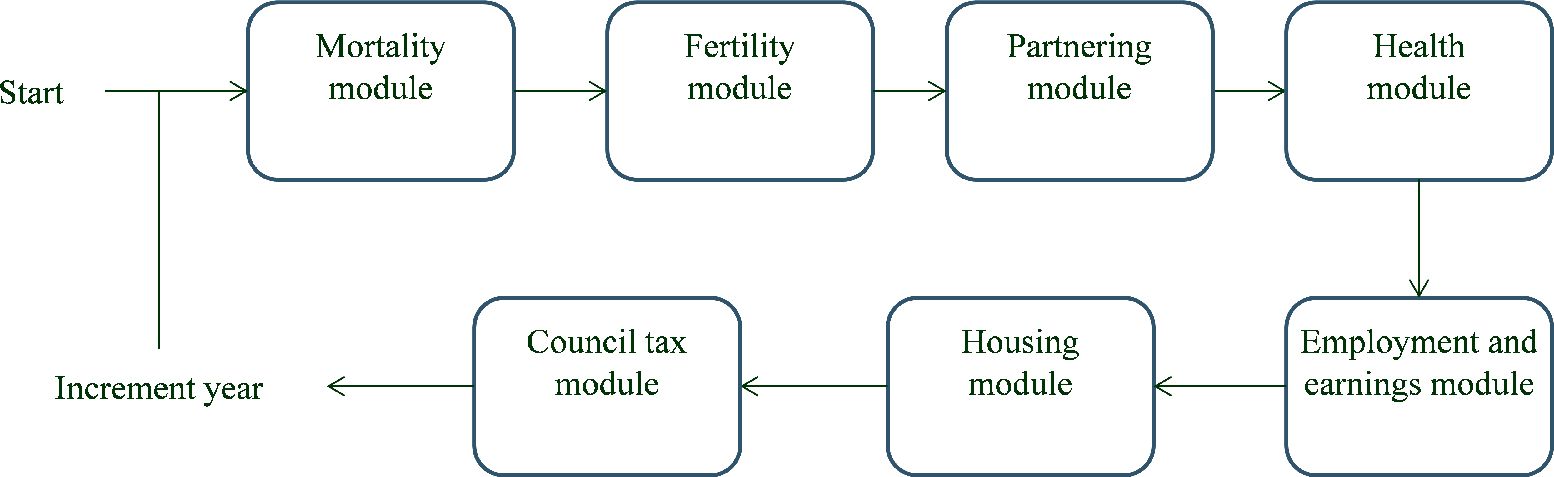
Figure 1

Microsimulation approach.
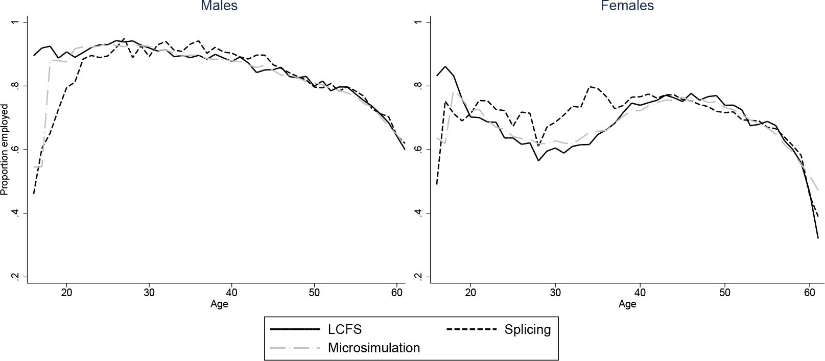
Figure 2

Employment: two approaches vs. LCFS, 1945–54 cohort.
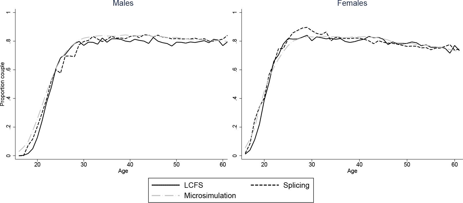
Figure 3
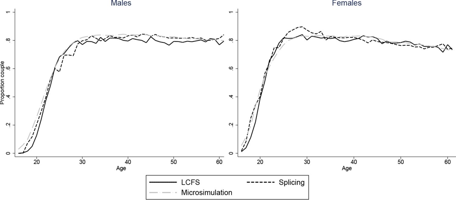
Proportion in couples: two approaches vs. LCFS, 1945–54 cohort.
Figure 4

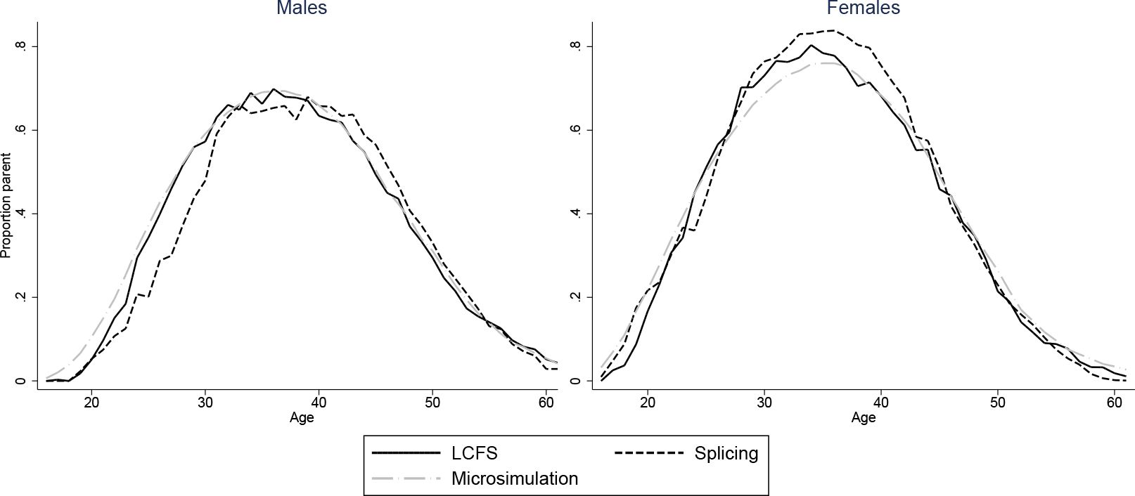
Proportion parents: two approaches vs. LCFS, 1945–54 cohort.
Figure 5

Proportion of parents that are single parents: two approaches vs. LCFS, 1945–54 cohort.
Figure 6

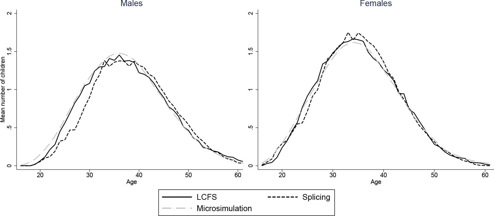
Number of children: two approaches vs. LCFS, 1945–54 cohort.
Figure 7

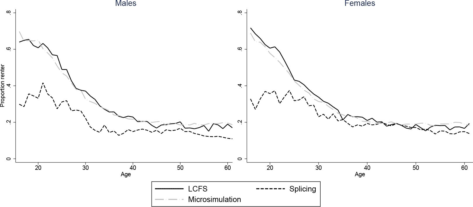
Proportion renters: two approaches vs. LCFS, 1945–54 cohort.
Figure 8
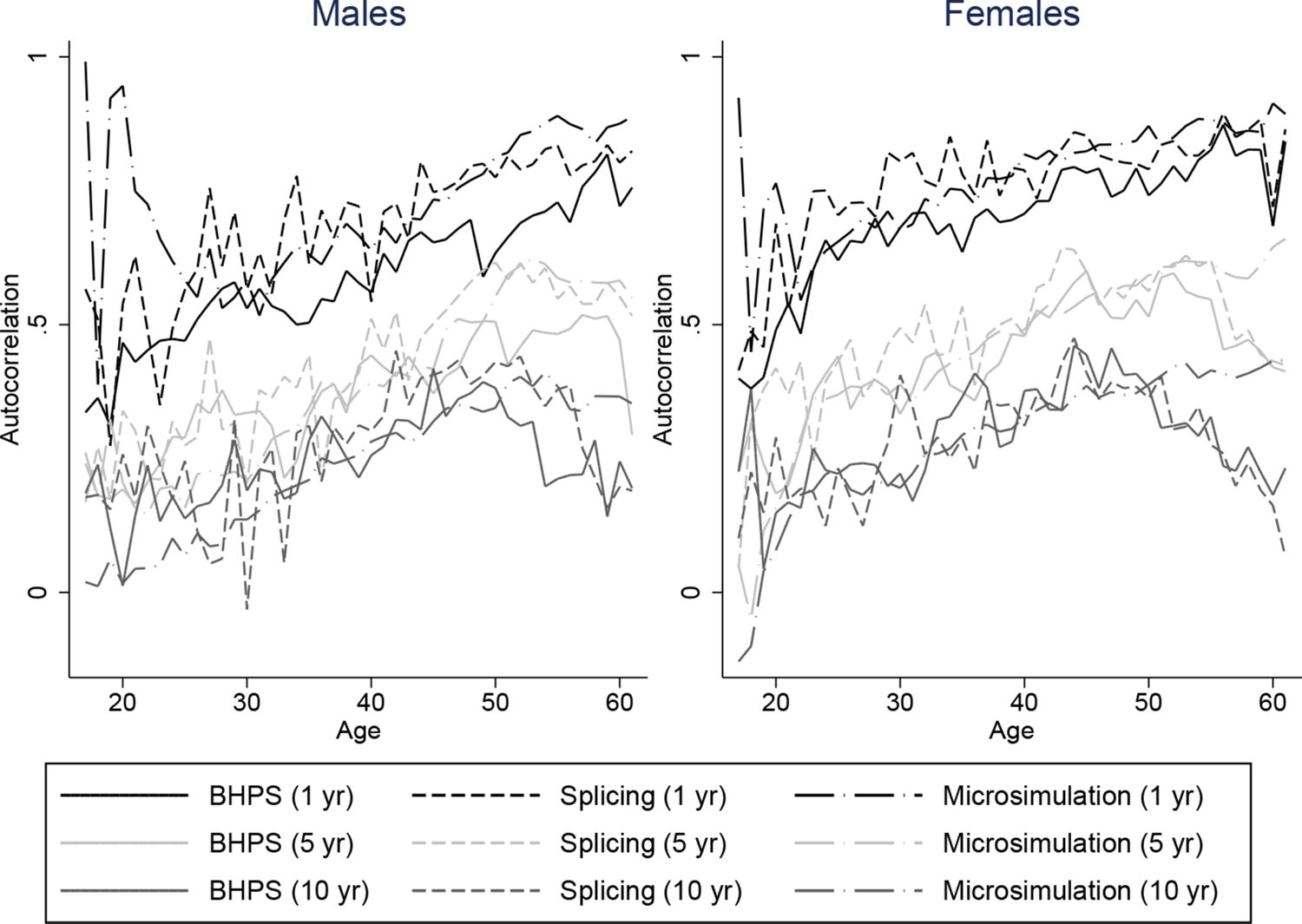
Autocorrelations for employment status: two approaches vs. BHPS, ages 16–65.
Figure 9
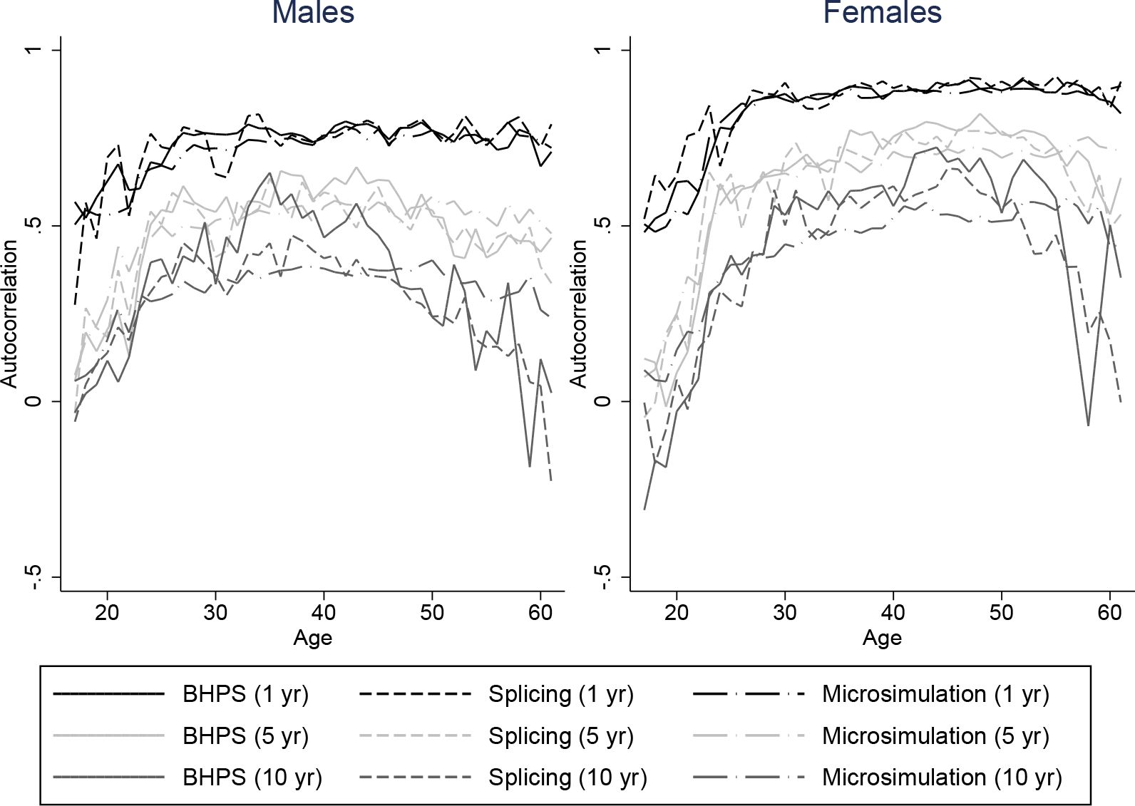

Autocorrelations in earnings ranks: two approaches vs. BHPS, ages 16–65.
Figure 10

Autocorrelations for couple status: two approaches vs. BHPS, ages 16–65.
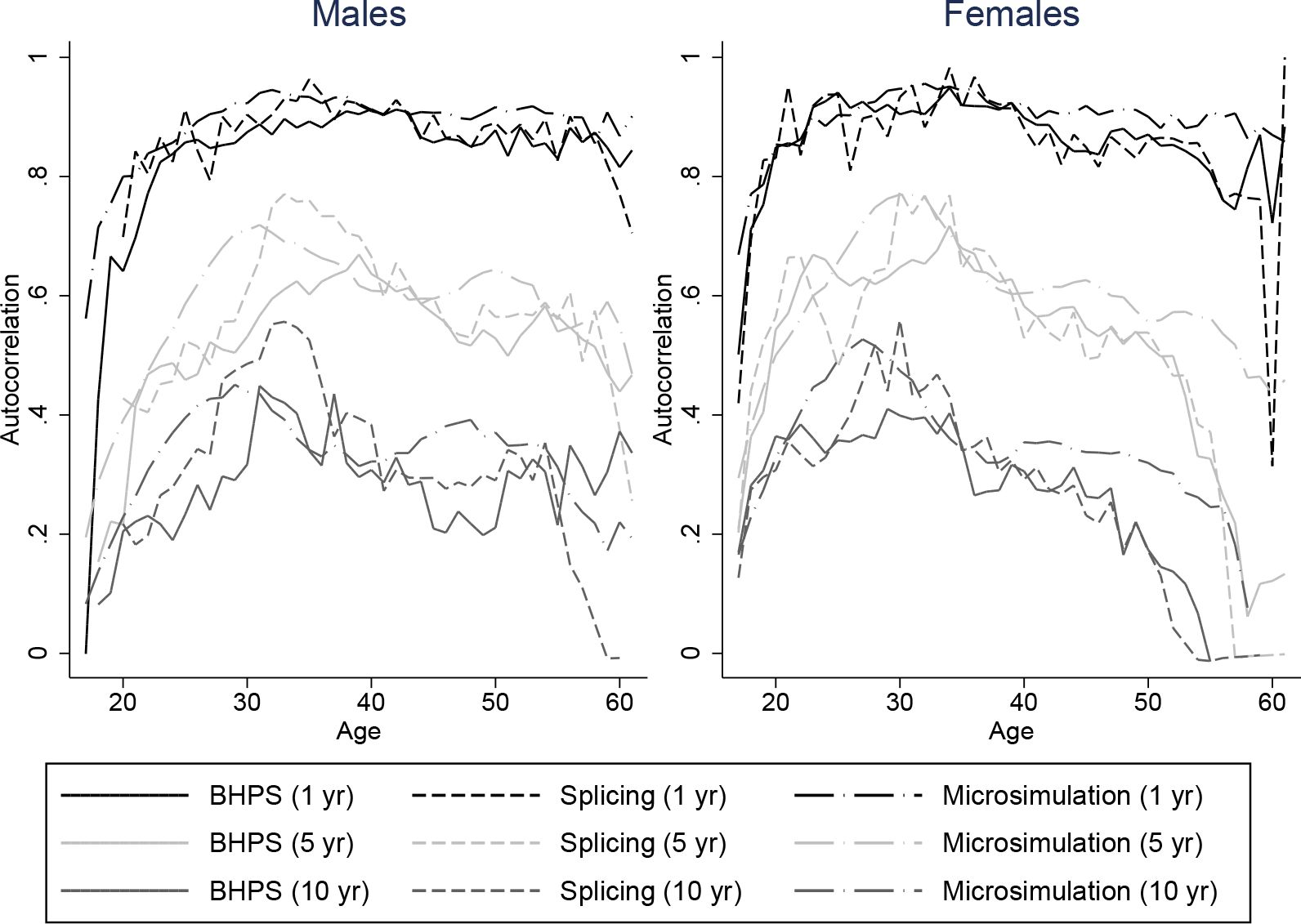
Figure 11

Autocorrelations for parent status: two approaches vs. BHPS, ages 16–65.
Tables
Table 1
Estimation equations.
| Outcome | Method | Subsamples | Independent variables |
|---|---|---|---|
| Mortality | Logit | Cubic in age, dummy for receipt of disability benefits, couple status, education dummies and earnings quintile | |
| Child arrival | LPM | Run separately for women in couples and single women | For childless women: quadratic in age, dummy for ever had kids, number of kids ever had For women in couples: as for childless but also banded number of kids (0,1,2, and 3 or more) in household, age of youngest child, age of youngest child interacted with age |
| Child departure | LPM | Run separately by age of child (16–19) | Dummies for mothers and fathers education |
| Partnering | Logit | Run separately for 3 education groups and sex | Quartic in age, dummy for employed last period, dummies for number of kids in household (0,1,and 2 or more), dummies for couple status in previous three periods, dummy for single status last period interacted with age |
| Separating | Logit | Run separately for own education and sex | Quartic in age, employed last period, partner employed last period, dummies for banded number of kids in household (0,1,and 2 or more), cubic in current relationship length, age of youngest child, dummy for education same as partner |
| Health (IB and DLA receipt) | Logit | For IB: quartic in age, 4 lags of employment status (interacted), 4 lags of IB status (interacted) earnings quartile last period For DLA: quartic in age, 4 lags of employment status (interacted), 4 lags of DLA status (interacted) earnings quartile last period and 2 lags of IB status | |
| Renter (21 and over) | Logit | Run separately for current owners and current renters and for over and under 21s | Age of head of household, education of head of household, earnings quintile last period of head of household, banded number of kids (0,1,2 or 3 or more), couple status, relationship length dummy for rented last period, 4 lags of ownership status |
| Rank in rent distribution (21 and over) | OL | Run separately for owners, and renters in each of 5 rent quintiles | Age of head of household, education of head of household, earnings quintile last period of head of household, banded number of kids (0,1,2 or 3 or more), couple status, relationship length dummy for rented last period, 4 lags of ownership status |
| Renter status and rank (under 21) | MNL | Age of head of household, Age of head of household squared, | |
| Council tax band | OL | Run separately for each of 8 possible prior bands | cubic in age, banded number of children (0,1,2,3, 4 or more) renter status earnings quartile of household head, employment status |
-
Notes: LPM = Linear probability model, OL = Ordered Logit, MNL = multinomial logit.
Table 2
Estimation equations for employment and earnings.
| Outcome | Method | Subsamples | Independent variables |
|---|---|---|---|
| Employment (22 and over) | Logit | Run separately for males and females, by employment in prior wave and by employment 2 waves ago | Education dummies, quartic in age, age-education interactions, dummy for over state pension age, dummy for having kids, dummy for couple status, dummy for having kids under 5, kids under 5 interacted with cubic in age, 3 lags of full-time status, banded number of kids (0,1,2 and 3 or more), couple status, couple-age interaction, lagged full-time status, lagged earnings rank,dummies for earnings quartiles (and 5 lags), employment status 3, 4,5 and 6 waves ago (and interactions), lagged disability status |
| Earnings quartile and part-time/full-time status (22 and over) | MNL | Run separately for each of 5 possible prior states: in part-time work, in full-time work and in 4 earnings quartiles and separately for males and females | Education dummies, quartic in age, age-education interactions, dummy for over state pension age, dummy for has kids, couple status, dummy for kids under 5, 3 lags of full-time status, current earnings rank (and 3 lags), 3 lags of earnings quartile dummies, 3 lags of employment status (interacted) |
| Employment and earnings (under 22) | MNL | Run separately for each of 6 prior possible states: unemployment, in part-time work, in full-time work and in 4 earnings quartiles | Sex, education dummies, dummy for has kids and age |
| Earnings rank within ‘bin’ (20 and over) | OLS | Run separately by prior state and sex | cubics in 4 lagged (within bin) ranks interacted with cubic in age, education dummies, dummies for ‘bin’ in previous 4 periods |
| Earnings rank within ‘bin’ (under 20) | OLS | Run separately by prior state and sex | cubics in lagged (within bin) ranks interacted with cubic in age, education dummies |
-
Notes: MNL = multinomial logit.
Table 3
Cells within which probabilities are matched to the LCFS.
| State | Cells |
|---|---|
| Couple | Age, year, sex, has children |
| Renter | Age, year |
| Employed | Age, year, sex, has children |
Table 4
Summary statistics (splicing approach).
| Number of synthetic life-cycles | 1,952 |
| Number of individuals used in splicing | 5,806 |
| Average number of splices per life-cycle | 8.48 |
| Average number of possible matches at joins | 35.4 |
| Proportion of years 16–83 (or death) covered | 88% |
| Completed until death | 514 |
Table 5
Autocorrelations in ranks for earnings.
| Age group | Autocorrelations when N match occurs | Autocorrelations when N no match occurs | ||
|---|---|---|---|---|
| 16–23 | 0.58 | 1,115 | 0.63 | 5,010 |
| 24–29 | 0.69 | 1,202 | 0.82 | 5,401 |
| 30–35 | 0.75 | 1,114 | 0.85 | 6,265 |
| 36–41 | 0.84 | 1,173 | 0.88 | 6,832 |
| 42–47 | 0.81 | 1,110 | 0.88 | 7,440 |
| 48–53 | 0.77 | 694 | 0.87 | 7,578 |
| 54–59 | 0.76 | 1,052 | 0.87 | 6,102 |
| 60–65 | 0.73 | 787 | 0.85 | 3,140 |
| 66–71 | 0.36 | 119 | 0.68 | 1,299 |
Table 6
Autocorrelations in ranks for partner’s earnings.
| Age group | Autocorrelations when N match occurs | Autocorrelations when N no match occurs | ||
|---|---|---|---|---|
| 16–23 | 0.45 | 410 | 0.66 | 1,228 |
| 24–29 | 0.64 | 998 | 0.78 | 4,046 |
| 30–35 | 0.76 | 913 | 0.86 | 5,261 |
| 36–41 | 0.67 | 1,015 | 0.83 | 5,829 |
| 42–47 | 0.78 | 924 | 0.83 | 6,041 |
| 48–53 | 0.75 | 560 | 0.80 | 6,312 |
| 54–59 | 0.67 | 832 | 0.80 | 4,862 |
| 60–65 | 0.50 | 526 | 0.73 | 2,493 |
| 66–71 | 0.34 | 134 | 0.68 | 969 |
Table 7
Autocorrelations in ranks for hours worked.
| Age group | Autocorrelations when N match occurs | Autocorrelations when N no match occurs | ||
|---|---|---|---|---|
| 16–23 | 0.39 | 1,310 | 0.47 | 6,115 |
| 24–29 | 0.37 | 1,321 | 0.65 | 5,752 |
| 30–35 | 0.61 | 1,188 | 0.74 | 6,618 |
| 36–41 | 0.65 | 1,224 | 0.75 | 7,183 |
| 42–47 | 0.61 | 1,152 | 0.74 | 7,752 |
| 48–53 | 0.60 | 730 | 0.72 | 7,924 |
| 54–59 | 0.68 | 1,085 | 0.76 | 6,363 |
| 60–65 | 0.58 | 811 | 0.76 | 3,351 |
| 66–71 | -0.02 | 151 | 0.63 | 1,418 |
Table 8
Autocorrelations in ranks for rent.
| Age group | Autocorrelations when N match occurs | Autocorrelations when N no match occurs | ||
|---|---|---|---|---|
| 16–23 | 0.54 | 529 | 0.70 | 2,324 |
| 24–29 | 0.69 | 446 | 0.82 | 1,893 |
| 30–35 | 0.40 | 295 | 0.78 | 1,418 |
| 36–41 | 0.37 | 226 | 0.78 | 1,334 |
| 42–47 | 0.61 | 259 | 0.77 | 1,477 |
| 48–53 | 0.70 | 195 | 0.79 | 1,476 |
| 54–59 | 0.50 | 180 | 0.77 | 1,209 |
| 60–65 | 0.50 | 142 | 0.78 | 980 |
| 66–71 | 0.63 | 103 | 0.76 | 558 |
Table 9
Persistence of employment and couple status for 1945–54 cohort in BHPS, spliced life-cycles, and simulations (1995–2004).
| BHPS | Splicing | Microsimulation | |
|---|---|---|---|
| Always employed | 55.9% | 55.8% | 56.3% |
| Always unemployed | 12.4% | 10.2% | 11.4% |
| Always couple | 73.7% | 73.7% | 73.6% |
| Always single | 15.6% | 15.1% | 12.9% |
| N | 676 | 1807 | 4666 |
-
Notes: BHPS probabilities weighted for probability of attrition.
Download links
A two-part list of links to download the article, or parts of the article, in various formats.