Linking CGE and microsimulation models: A comparison of different approaches
- Department of Economic and Social Science - Catholic University of Milan and SiNSYS NV/SA
- Article
- Figures and data
- Jump to
Figures

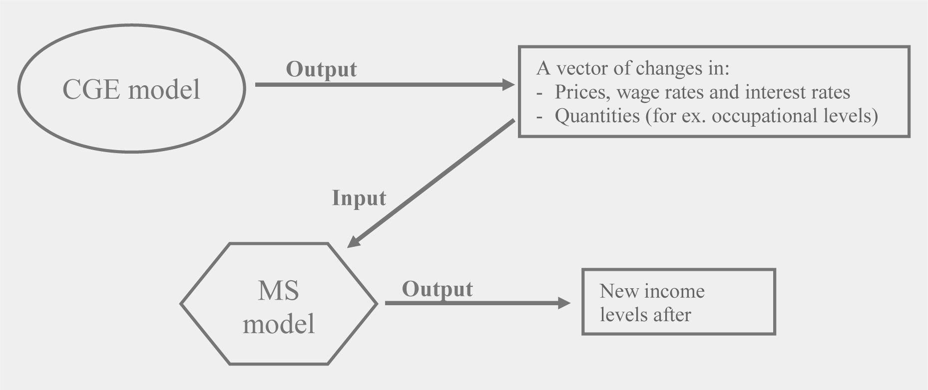
The Top-Down approach.

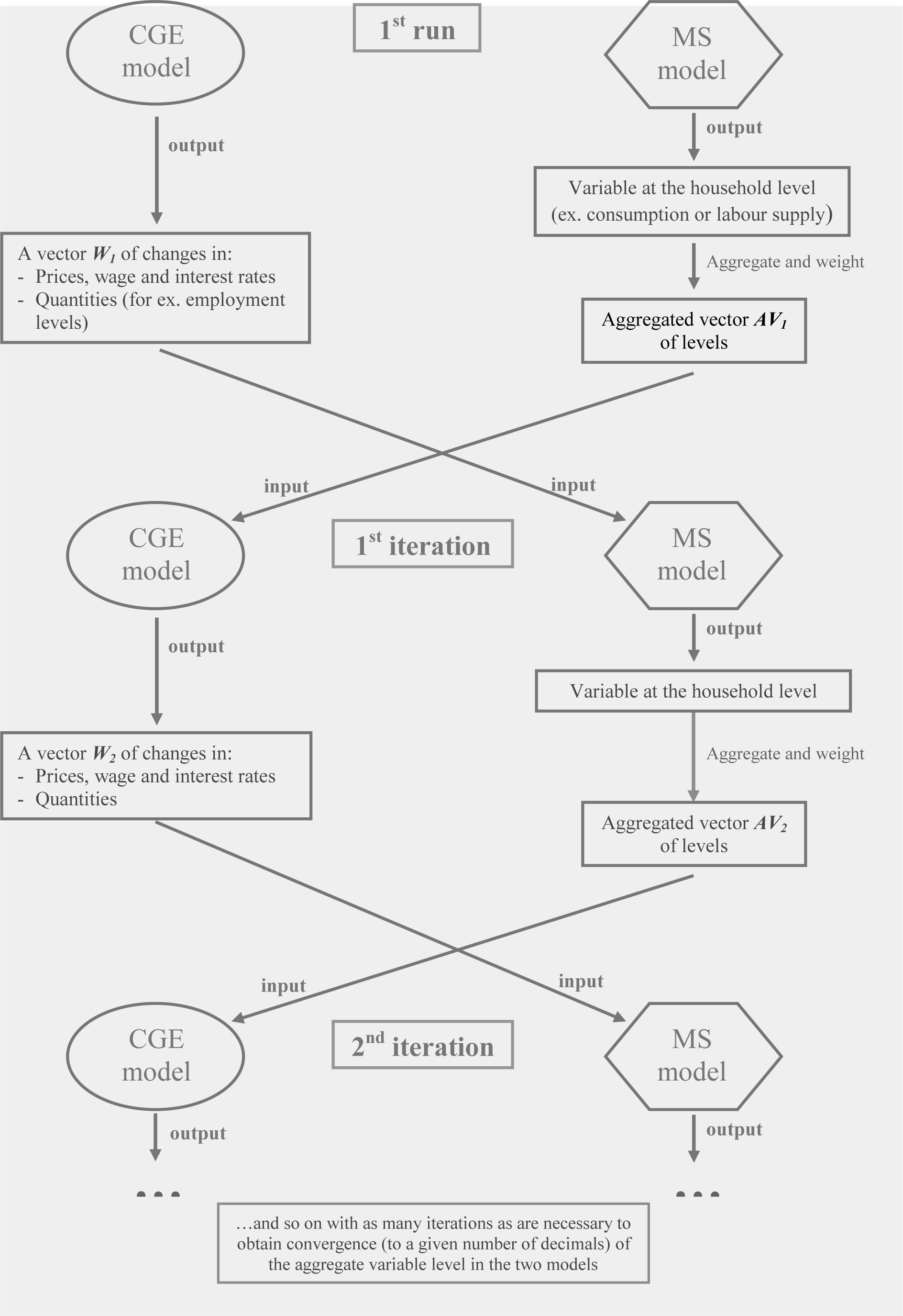
The Top-Down/Bottom-Up approach.
Tables
Description of the subscripts for the microsimulation model.
| m | Households | m = 1, 2, …, 24 | |
| i | Individuals belonging to household m | i = 1, …, NCm | (NCm: number of components of household m) |
| q | Goods | q = 1,2 |
Direct income tax rates.
| Household Income | Tax rate |
|---|---|
| Up to 10,000 | 0% |
| Up to 15,000 | 15% |
| Up to 26,000 | 24% |
| Up to 70,000 | 32% |
| Over 70,000 | 39% |
Heckman selection model, two-step estimates.
| Coefficient | Std. Error | z | P>|z| | |
|---|---|---|---|---|
| constant | 7.0321 | 0.3145 | 22.36 | 0.000 |
| ln(age) | 0.6978 | 0.0833 | 8.38 | 0.000 |
| sex | −0.4662 | 0.1018 | −4.58 | 0.000 |
| qualification | 0.3966 | 0.0772 | 5.14 | 0.000 |
| education | 0.5250 | 0.0872 | 6.02 | 0.000 |
| Mills ratio | 0.2160 | 0.1473 | 1.47 | 0.143 |
| Selection | ||||
| ln(age) | 0.3386 | 0.0807 | 4.19 | 0.000 |
| sex | −1.5492 | 0.2803 | −5.53 | 0.000 |
| qualification | 1.0204 | 0.2729 | 3.74 | 0.000 |
| children under 6 | 0.1682 | 0.2368 | 0.71 | 0.478 |
| region | −0.7515 | 0.2980 | −2.52 | 0.012 |
| rho | 0.7628 | |||
| sigma | 0.2832 |
-
Notes: Dependent variable: logarithm of wage.
Binary logit model of labour status choice.
| Coefficient | Std. Error | z | P>|z| | |
|---|---|---|---|---|
| ln(real wage) | 0.1972 | 0.0465 | 4.25 | 0.000 |
| sex | −1.8948 | 0.4078 | −4.65 | 0.000 |
| qualification | 1.4408 | 0.4257 | 3.38 | 0.001 |
| region | −0.7185 | 0.3295 | −2.18 | 0.029 |
| children under 6 | 0.2691 | 0.2973 | 0.91 | 0.365 |
| education | −0.7633 | 0.6717 | −1.14 | 0.256 |
| Mean dependent var | 0.6647 | S.D. dependent var | 0.4735 | |
| S.E. of regression | 0.3767 | Akaike info criterion | 0.9015 | |
| Sum squared resid | 23.2688 | Schwarz criterion | 1.0122 | |
| Log likelihood | −70.6305 | Hannan-Quinn criter. | 0.9464 | |
| Avg. log likelihood | −0.4155 | |||
-
Notes: Dependent Variable: Activity Status.
SAM of the economy.
| C1 | C2 | S1 | S2 | K | L | H | G | SI | RoW | Total | |
|---|---|---|---|---|---|---|---|---|---|---|---|
| C1 | 57.5 | 15.5 | 95.2 | 61.2 | 30.3 | 23.5 | 283.3 | ||||
| C2 | 17.1 | 23.5 | 312.8 | 48.5 | 14.2 | 76.5 | 492.5 | ||||
| S1 | 283.3 | 283.3 | |||||||||
| S2 | 492.5 | 492.5 | |||||||||
| K | 72.2 | 23.0 | 13.1 | 108.3 | |||||||
| L | 83.2 | 353.8 | 116.4 | 553.4 | |||||||
| H | 108.3 | 553.4 | 39.8 | 701.5 | |||||||
| G | 12.3 | 17.7 | 249.0 | 279.0 | |||||||
| SI | 44.5 | 44.5 | |||||||||
| RoW | 41.0 | 59.0 | 100.0 | ||||||||
| Total | 283.3 | 492.5 | 283.3 | 492.5 | 108.3 | 553.4 | 701.5 | 269.9 | 44.5 | 100.0 |
-
Notes: Cq: consumption of good q; Sq: production sector q; K: capital account; L: labour account; H: representative household account; G: public sector; SI: savings-investments account, RoW: Rest of the World account.
Values of some parameters for the CGE model.
| Sector 1 | Sector 2 | |
|---|---|---|
| Elasticity of substitution (EOS) in production function (aggregation of capital and labour) | 0.7 | 0.5 |
| Elasticity of substitution for Armington composite good | 0.7 | 1.2 |
| Elasticity of transformation for exports and domestic production delivered to the domestic market | −2.0 | −3.0 |
| Initial tariff rates on imports | 0.3 | 0.3 |
| Initial time endowment | 656.7 | |
| Wage elasticity of labour supply (estimated from the household survey) | −0.18665 |
Variables and parameters of the CGE model
| Variables | Parameters | ||
|---|---|---|---|
| PK | Return to capital | ty | Income tax rate |
| PL | Wage rate | tmq | Tariff rates on imports |
| Pq | Price of Armington composite good | ε_LS | Wage elasticity of labour supply |
| PDq | Price of output | mps | Marginal propensity to save |
| PDDq | Price of domestically produced good delivered to domestic market | αHq | Cobb-Douglas power of commodity q in RH’s utility function |
| PWEq | World price of exports (foreign currency) | αHl | Cobb-Douglas power of leisure in RH’s utility function |
| PWMq | World price of imports (foreign currency) | αCGq | Cobb-Douglas power of commodity q in government utility function |
| PMq | Price of imports (local currency) | αKG | Cobb-Douglas power of capital in government utility function |
| PEq | Price of exports (local currency) | αLG | Cobb-Douglas power of labour in government utility function |
| ER | Exchange rate | ioqs | Technical coefficients |
| PC | Consumer price index | aFq | Efficiency parameter production function |
| KS | Capital endowment (exogenous) | γFq | Share parameter in production function |
| LS | Labour supply (endogenous) | σFq | EOS in firm q’s production function |
| TS | Time endowment (exogenous) | aAq | Efficiency parameter in Armington function |
| Xq | Domestic sales (Armington composite) | γAq | Share parameter in Armington function |
| XDq | Domestic production | σAq | EOS in firm q’s Armington function |
| XDDq | Domestically produced good delivered to domestic market | αIq | Cobb-Douglas power of commodity q in Bank’s utility function |
| Mq | Imports | aTq | Efficiency parameter in CET function |
| Eq | Exports | γTq | Share parameter in CET function |
| Kq | Capital demand by firms | σTq | Elasticity of transformation in CET function |
| Lq | Labour demand by firms | ||
| Iq | Investment good | ||
| Cq | Consumption demand by household | ||
| Cl | Demand for leisure | ||
| Y | Household’s income | ||
| S | Household’s savings | ||
| CBUD | Household’s consumption expenditure | ||
| TF | Public transfers to household | ||
| TAXREV | Tax revenues | ||
| CGq | Consumption demand by government | ||
| KG | Capital demand by government | ||
| LG | Labour demand by government | ||
Equations of the CGE model
| Description | Equations |
|---|---|
| Demand for consumption goods | |
| Leisure | |
| Labour supply | |
| Savings | |
| Consumer price index | |
| CES production function | |
| CES FOC for capital | |
| Demand for investment goods | |
| Price of imports in local currency | |
| Price of exports in local currency | |
| Armington function | |
| Armington FOC for imports | |
| CET function | |
| CET FOC for exports | |
| Market clearing condition for labour | |
| Market clearing condition for capital | |
| Market clearing condition for commodity q | |
| Income definition | |
| Disposable income minus savings | |
| Zero profit condition in production function | |
| Zero profit condition in Armington function | |
| Zero profit condition in CET function | |
| Demand of commodity q by government | |
| Demand of capital by government | |
| Demand of labour by government | |
| Tax revenues |
Simulation results: percentage changes (CGE model).
| Integrated Approach | Top-Down Approach | TD/BU Approach (C&LS) | TD/BU Approach (LS) | |
|---|---|---|---|---|
| Government Surplus | 0.00 | 0.00 | 0.00 | 0.00 |
| Wage Rate | −14.87 | −14.67 | −14.42 | −14.64 |
| Capital Return | 19.70 | 19.30 | 17.91 | 19.13 |
| Consumer Price Index | 0.00 | 0.00 | 0.00 | 0.00 |
| Exchange Rate | 53.83 | 53.76 | 53.83 | 53.70 |
| Labour Supply | −1.00 | −1.18 | −1.32 | −1.32 |
| Government Use of Labour | 4.82 | 4.23 | 3.72 | 4.06 |
| Government Use of Capital | −25.45 | −25.45 | −24.72 | −25.43 |
| Income* | −9.50 | −9.39 | −9.50 | −9.48 |
| Disposable Income* | −9.50 | −9.39 | −9.50 | −9.48 |
| Consumption Expenditure* | −9.50 | −9.39 | −7.90 | −9.48 |
| Marginal Propensity to Save | 0.00 | 0.00 | −16.22 | 0.00 |
| Savings* | −9.28 | −9.39 | −24.18 | −9.48 |
| Tax Revenues | −9.28 | −9.48 | −9.63 | −9.58 |
-
*
For the integrated model, these changes are computed as average percentage changes across households.
Simulation results: percentage changes (CGE model).
| Macro variables | Integrated Approach | Top-Down Approach | TD/BU Approach (C&LS) | TD/BU Approach (LS) | ||||
|---|---|---|---|---|---|---|---|---|
| Sector 1 | Sector 2 | Sector 1 | Sector 2 | Sector 1 | Sector 2 | Sector 1 | Sector 2 | |
| Commodity Prices | −0.99 | 0.30 | −1.23 | 0.38 | −1.70 | 0.52 | −1.27 | 0.39 |
| Domestic Sales | −8.69 | −12.52 | −8.81 | −12.54 | −10.21 | −12.05 | −8.88 | −12.64 |
| Domestic Production | 27.81 | −14.20 | 27.91 | −14.31 | 26.77 | −13.86 | 27.84 | −14.43 |
| Labour Demand | 43.52 | −13.22 | 43.05 | −13.36 | 41.08 | −12.94 | 42.88 | −13.48 |
| Capital Demand | 13.07 | −26.82 | 13.14 | −26.72 | 12.72 | −25.84 | 13.15 | −26.76 |
| Consumption* | −8.60 | −9.78 | −8.26 | −9.73 | −6.58 | −8.30 | −8.32 | −9.84 |
| Investment | −7.65 | −8.84 | −8.26 | −9.73 | −22.87 | −24.57 | −8.32 | −9.84 |
| Imports | −32.92 | −47.63 | −33.11 | −47.57 | −34.37 | −47.21 | −33.16 | −47.60 |
| Exports | 207.36 | −78.38 | 209.23 | −78.53 | 209.10 | −78.48 | 209.11 | −78.59 |
-
*
For the integrated model, these changes are computed as average percentage changes across households.
Simulation results: Inequality indices on disposable per capita real income (MS model).
| Benchmark Values | Integrated Approach* | Top-Down Approach* | TD/BU Approach (C & LS)* | TD/BU Approach (LS)* | |
|---|---|---|---|---|---|
| Gini Index | 31.85 | 3.02% | 1.68% | 1.52% | 1.66% |
| Atkinson’s Index, ε = 0.5 | 8.46 | 4.94% | 3.01% | 2.72% | 2.97% |
| Coefficient of Variation | 65.86 | 3.78% | 2.84% | 2.64% | 2.81% |
| Generalized Entropy Measures: | |||||
| I(c), c = 2 | 21.69 | 7.69% | 5.75% | 5.35% | 5.70% |
| Mean Logarithmic Deviation, I(0) | 17.72 | 3.99% | 2.10% | 1.83% | 2.07% |
| Theil Coefficient, I(1) | 17.82 | 5.89% | 3.89% | 3.58% | 3.85% |
-
*
Percentage deviations from benchmark values.
Simulation results: Poverty indices on disposable per capita real income (MS model).
| Benchmark Values | Integrated Approach* | Top-Down Approach* | TD/BU Approach (C & LS)* | TD/BU Approach (LS)* | |
|---|---|---|---|---|---|
| General Poverty Line | |||||
| Headcount Index, P0 | 40.98 | 56.00% | 8.00% | 8.00% | 8.00% |
| Poverty Gap Index, P1 | 9.84 | 119.46% | 27.25% | 27.01% | 27.21% |
| Poverty Severity Index, P2 | 0.00 | 143.04% | 28.95% | 28.51% | 28.88% |
| Extreme Poverty Line | |||||
| Headcount Index, P0 | 4.92 | 166.67% | 33.33% | 33.33% | 33.33% |
| Poverty Gap Index, P1 | 1.00 | 71.09% | 4.77% | 4.64% | 4.75% |
| Poverty Severity Index, P2 | 0.00 | 45.33% | −0.03% | 0.03% | −0.03% |
-
*
Percentage deviations from benchmark values.
SAM of the economy made consistent with the Household Survey.
| C1 | C2 | S1 | S2 | K | L | H | G | SI | RoW | Total | |
|---|---|---|---|---|---|---|---|---|---|---|---|
| C1 | 57.8 | 15.6 | 95.4 | 62.6 | 28.1 | 23.6 | 283.0 | ||||
| C2 | 17.1 | 23.5 | 313.2 | 48.8 | 13.6 | 76.6 | 492.8 | ||||
| S1 | 283.3 | 283.0 | |||||||||
| S2 | 492.5 | 492.8 | |||||||||
| K | 73.4 | 23.2 | 13.2 | 109.8 | |||||||
| L | 81.7 | 353.8 | 117.5 | 552.6 | |||||||
| H | 109.8 | 552.6 | 38.7 | 701.2 | |||||||
| G | 12.3 | 17.7 | 250.8 | 280.8 | |||||||
| SI | 41.7 | 41.7 | |||||||||
| RoW | 40.8 | 59.4 | 100.2 | ||||||||
| Total | 283.0 | 492.8 | 283.0 | 492.8 | 109.8 | 552.6 | 701.2 | 280.8 | 41.7 | 100.2 |
-
Notes: Cq: consumption of good q; Sq: production sector q; K: capital account; L: labour account; H: representative household account; G: public sector; SI: savings-investments account, RoW: Rest of the World account.
Simulation results with consistent data: Percentage changes (CGE model).
| TD/BU Approach (C & LS) | TD/BU Approach (LS) | |
|---|---|---|
| Government Surplus | 0.00 | 0.00 |
| Wage Rate | −14.63 | −14.81 |
| Capital Return | 18.36 | 19.37 |
| Consumer Price Index (num.) | 0.00 | 0.00 |
| Exchange Rate | 53.90 | 53.80 |
| Labour Supply | −1.18 | −1.18 |
| Government Use of Labour | 4.13 | 4.42 |
| Government Use of Capital | −24.89 | −25.48 |
| Income | −9.45 | −9.43 |
| Disposable Income | −9.45 | −9.43 |
| Consumption Expenditure | −8.14 | −9.43 |
| Marginal Propensity to Save | −14.13 | 0.00 |
| Savings | −22.24 | −9.43 |
| Tax Revenues | −9.57 | −9.52 |
Simulation results with consistent data: Percentage changes (CGE model).
| TD/BU Approach (C & LS) | TD/BU Approach (LS) | |||
|---|---|---|---|---|
| Sec 1 | Sec 2 | Sec 1 | Sec 2 | |
| Commodity Prices | −1.44 | 0.44 | −1.07 | 0.33 |
| Domestic Sales | −9.86 | −12.06 | −8.89 | −12.55 |
| Domestic Production | 26.77 | −13.80 | 27.65 | −14.27 |
| Labour Demand | 41.65 | −12.85 | 43.17 | −13.30 |
| Capital Demand | 12.70 | −25.99 | 13.05 | −26.76 |
| Consumption | −7.13 | −8.45 | −8.45 | −9.73 |
| Investment | −21.11 | −22.58 | −8.45 | −9.73 |
| Imports | −34.12 | −47.30 | −33.10 | −47.63 |
| Exports | 207.50 | −78.34 | 207.46 | −78.43 |
TD/BU-C&LS approach with consistent data: RH shares from CGE model used in the MS model (percentage changes, CGE model).
| only ty | only ΔLS | only ηi & mps | ΔLS, ty, mps & ηi | |
|---|---|---|---|---|
| Marginal propensity to save Savings | 2.92 | −14.82 | −14.47 | 0.12 |
| Savings | −6.78 | −22.87 | −22.55 | −9.33 |
Simulation results TD/BU approach: percentage changes (CGE model).
| ΔLS & ty (inconsistent data) | ΔLS, ty, mps & ηi (inconsistent data) | ΔLS, ty, mps & ηi (consistent data) | |
|---|---|---|---|
| Government Surplus | 0.00 | 0.00 | 0.00 |
| Wage Rate | −14.70 | −14. 62 | −14.84 |
| Capital Return | 19.43 | 18.95 | 19.46 |
| Consumer Price Index (num.) | 0.00 | 0.00 | 0.00 |
| Exchange Rate | 53.90 | 53.95 | 54.02 |
| Labour Supply | −1.18 | −1.18 | −1.18 |
| Government Use of Labour | 2.26 | 2.13 | 1.62 |
| Government Use of Capital | −26.96 | −26.69 | −27.55 |
| Income | −9.39 | −9.40 | −9.44 |
| Disposable Income | −8.47 | −8.48 | −8.12 |
| Consumption Expenditure | −8.47 | −7.93 | −8.14 |
| Marginal Propensity to Save | 0.00 | −5.53 | 0.25 |
| Savings | −8.47 | −13.54 | −7.89 |
| Tax Revenues | −10.95 | −10.97 | −11.60 |
Simulation results TD/BU approach: percentage changes (CGE model).
| ΔLS & ty (inconsistent data) | ΔLS, ty, mps & ηi (inconsistent data) | ΔLS, ty, mps & ηi (consistent data) | ||||
|---|---|---|---|---|---|---|
| Sec 1 | Sec 2 | Sec 1 | Sec 2 | Sec 1 | Sec 2 | |
| Commodity Prices | −1.21 | 0.37 | −1.38 | 0.42 | −1.09 | 0.33 |
| Domestic Sales | −8.75 | −12.00 | −9.27 | −11.77 | −8.92 | −11.73 |
| Domestic Production | 28.13 | −13.75 | 27.72 | −13.53 | 27.87 | −13.42 |
| Labour Demand | 43.37 | −12.79 | 42.66 | −12.58 | 43.46 | −12.44 |
| Capital Demand | 13.28 | −26.30 | 13.11 | −25.93 | 13.20 | −26.07 |
| Consumption | −7.35 | −8.81 | −6.90 | −8.24 | −7.45 | −8.35 |
| Investment | −7.35 | −8.81 | −12.33 | −13.91 | −6.88 | −8.19 |
| Imports | −33.09 | −47.31 | −33.57 | −47.16 | −33.20 | −47.23 |
| Exports | 210.17 | −78.31 | 210.17 | −78.27 | 208.79 | −78.11 |
Simulation results TD/BU approach: percentage changes (MS model).
| ΔLS & ty (inconsistent data) | ΔLS, ty, mps & ηi (inconsistent data) | TD Approach (inconsistent data) | ||||
|---|---|---|---|---|---|---|
| Sec 1 | Sec 2 | Sec 1 | Sec 2 | Sec 1 | Sec 2 | |
| Consumption | −7.23 | −8.28 | −7.45 | −8.35 | −7.21 | −8.28 |
| Savings | −7.78 | −7.88 | −7.78 | |||
Inequality indices on disposable per capita real income (MS model).
| Benchmark Values | ΔLS & ty (inconsistent data)* | ΔLS, ty, mps & ηi (consistent data)* | |
|---|---|---|---|
| Gini Index | 31.85 | 1.70% | 1.66% |
| Atkinson’s Index, ε = 0.5 | 8.46 | 3.04% | 2.97% |
| Coefficient of Variation | 65.86 | 2.86% | 2.81% |
| Generalized Entropy Measures: | |||
| I(c), c = 2 | 21.69 | 5.80% | 5.70% |
| Mean Logarithmic Deviation, I(0) | 17.72 | 2.13% | 2.07% |
| Theil Coefficient, I(1) | 17.82 | 3.93% | 3.85% |
-
*
Percentage deviations from benchmark values
Poverty indices on disposable per capita real income (MS model).
| Benchmark Values | ΔLS & ty (inconsistent data)* | ΔLS, ty, mps & ηi (consistent data)* | |
|---|---|---|---|
| General Poverty Line | |||
| Headcount Index, P0 | 40.98 | 8.00% | 8.00% |
| Poverty Gap Index, P1 | 9.84 | 27.30% | 27.21% |
| Poverty Severity Index, P2 | 0.00 | 29.01% | 28.88% |
| Extreme Poverty Line | |||
| Headcount Index, P0 | 4.92 | 33.33% | 33.33% |
| Poverty Gap Index, P1 | 1.00 | 4.79% | 4.75% |
| Poverty Severity Index, P2 | 0.00 | −0.03% | −0.03% |
-
*
Percentage deviations from benchmark values